Research Article
Patient-Specific Phantomless Estimation of Bone Mineral
Density and Its Effects on Finite Element Analysis Results: A
Feasibility Study
Young Han Lee ,
1Jung Jin Kim ,
2and In Gwun Jang
21Department of Radiology, College of Medicine, 50-1 Yonsei-ro, Seodaemun-gu, Seoul 03722,
Yonsei University College of Medicine, Republic of Korea
2The Cho Chun Shik Graduate School of Green Transportation, 291, Daehak-ro, Yuseong-gu, Daejeon 34141,
Korea Advanced Institute of Science and Technology, Republic of Korea
Correspondence should be addressed to In Gwun Jang; [email protected]
Received 15 June 2018; Revised 6 November 2018; Accepted 6 December 2018; Published 3 January 2019 Academic Editor: Maria E. Fantacci
Copyright © 2019 Young Han Lee et al. This is an open access article distributed under the Creative Commons Attribution License, which permits unrestricted use, distribution, and reproduction in any medium, provided the original work is properly cited.
Objectives. This study proposes a regression model for the phantomless Hounsfield units (HU) to bone mineral density (BMD)
conversion including patient physical factors and analyzes the accuracy of the estimated BMD values. Methods. The HU values, BMDs, circumferences of the body, and cross-sectional areas of bone were measured from 39 quantitative computed tomography images of L2 vertebrae and hips. Then, the phantomless HU-to-BMD conversion was derived using a multiple linear regression model. For the statistical analysis, the correlation between the estimated BMD values and the reference BMD values was evaluated using Pearson’s correlation test. Voxelwise BMD and finite element analysis (FEA) results were analyzed in terms of root-mean-square error (RMSE) and strain energy density, respectively. Results. The HU values and circumferences were statistically significant (p < 0.05) for the lumbar spine, whereas only the HU values were statistically significant (p < 0.05) for the proximal femur. The BMD values estimated using the proposed HU-to-BMD conversion were significantly correlated with those measured using the reference phantom: Pearson’s correlation coefficients of 0.998 and 0.984 for the lumbar spine and proximal femur, respectively. The RMSEs of the estimated BMD values for the lumbar spine and hip were 4.26 ± 0.60 (mg/cc) and 8.35 ± 0.57 (mg/ cc), respectively. The errors of total strain energy were 1.06% and 0.91%, respectively. Conclusions. The proposed phantomless HU-to-BMD conversion demonstrates the potential of precisely estimating BMD values from CT images without the reference phantom and being utilized as a viable tool for FEA-based quantitative assessment using routine CT images.
1. Introduction
Osteoporosis is a common metabolic bone disorder that leads to increased bone fracture risk. As the elderly pop-ulation increases, the prevalence of osteoporosis is steadily increasing [1, 2]; thus, bone strength assessment has be-come more important as a diagnosis tool for osteoporosis. In principle, bone strength depends on two parameters: bone quality (e.g., bone architecture) and bone quantity (e.g., bone mineral density). In clinical practice, the esti-mation of bone strength has been based on the repre-sentative areal bone mineral density (aBMD) for the region of interest obtained by dual energy X-ray absorptiometry
(DXA) [3–5]. However, the representative aBMD cannot be a perfect stand-alone measure of bone strength because it neglects the 3D bone structure. It has been reported that two individuals who have identical bone density can have different fracture risks due to different bone structures [6]. In contrast to representative aBMDs, voxelwise volu-metric BMDs (vBMDs), which can be obtained using quantitative computed tomography (QCT) [7, 8], can provide a spatial BMD distribution in 3D, thereby elimi-nating the aforementioned sources of errors in estimating bone strength. In order to precisely measure the BMD values, QCT examination requires a reference phantom that is constructed from K2HPO4with known densities [9, 10].
Volume 2019, Article ID 4102410, 10 pages https://doi.org/10.1155/2019/4102410
The existence of a reference phantom eliminates potential confounding factors from scattering and beam hardening, which depend on individual patient factors such as waist circumference and weight. QCT also excludes osteophytes [11] and aortic/vascular calcifications [12], which might affect BMD. For the lumbar spine and proximal femur in which trabecular bone is prevalent, QCT can provide a diagnostic sensitivity for osteoporosis diagnosis greater than that using DXA [12].
In particular, QCT-based finite element analysis (FEA), which uses the 3D geometry and spatial BMD distribution of a target bone measured from the QCT examination, enables the precise estimation of patient-specific bone strength [13–15]. This quantitative approach has been proven to estimate fracture loads and sites [16–18]. It should be em-phasized that the measurement of voxelwise BMD is critical to conduct a reliable FEA because the elastic moduli of each finite element need to be derived through the BMD-modulus relationship [12, 16–18]. For precise voxelwise BMD mea-surement, however, a reference phantom must be placed below the patient during scanning, thereby causing addi-tional expenses and logistical burden in clinical imaging. Because routine CT scans (i.e., phantomless CT scans) are acquired for various purposes in clinical practice, it would be useful to be able to estimate the voxelwise BMD values using these routine CTscans without additional QCTexamination. To date, several Hounsfield unit (HU) to BMD con-version methods have been introduced [19–22]. Because BMD values are significantly related to HU values [23], the various effects of scanning protocol on HU values have been further investigated: contrast-enhanced CT [21, 22], CT colonography [24, 25], abdominal multi-detector CT [20], and spine CT [19, 22]. These studies have demonstrated that the correlation between the HU and BMD values depends on the contrast medium [25, 26], on kVp [27], and on the CT scanning regions. It is noteworthy that patient physical factors such as waist circumference must be considered for accurate phantomless HU-to-BMD conversions because these factors can affect the attenuation of radiation and therefore the HU values. However, few works in the liter-ature to date have addressed the effects of patient physical factors on the HU-to-BMD conversion and its subsequent impact on FEA-based quantitative assessment.
Therefore, for the lumbar spine and proximal femur, this study (1) proposes the phantomless HU-to-BMD conversion equations that consider the circumference and bone area as patient-specific physical factors, (2) investigates the corre-lation of BMD values between the proposed phantomless conversion and the reference phantom-based measurement, and (3) analyzes the accuracy of the estimated BMD values in terms of voxelwise BMD and FEA.
2. Materials and Methods
2.1. Study Population. The study population was
retro-spectively identified using the hospital information system. The inclusion criteria were (1) QCT examination conducted in April 2014 and (2) no bony abnormalities on the ra-diologic report. For a total of 39 identified cases, the
purposes of the QCT examination were medical check-up (n � 36), breast cancer follow-up (n � 1), and thyroid cancer follow-up (n � 2). The gender distribution was 14 males and 25 females. The mean age was 49.1 years (age 30–73). The inclusion criteria were QCT examination and no bony ab-normalities on the radiologic report. This retrospective study was approved by the hospital’s Institutional Review Board (IRB).
2.2. Image Protocol. QCT scans were performed in a
64-channel CT (Somatom definition AS+, Siemens, Erlangen, Germany), of which quality control and assessment are routinely performed every three months. The CT scan pa-rameters were optimized for QCT examination as follows: 120 kVp, 150 effective mAs, beam collimation � 20 mm, rotation speed � 0.6 seconds, pitch � 1.0 : 1, 512 × 512 matrix, field of view (FOV) � 360 mm, slice thickness � 3 mm, and reconstruction with B40s medium. The CARE Dose 4D and CARE kV were off. The CT dose index (CTDI 32 cm) was 10.10 mGy, and the dose length product (DLP) was 218.7 mGy·cm. Deep-inspiration breath-hold method was used for the QCT scans. All QCT scans were done with no contrast media.
2.3. Calculation of the Reference BMD Values Using the Reference Phantom. Five regions of interest (ROIs) for the
five different mineral contents of the reference phantom (Mindways Inc., Austin, TX, USA) were recorded in the same CT images. For the CT image of each patient, the phantom-based calibration algorithm [28, 29] determined the linear correlation between the known mineral densities and their corresponding HU values as follows:
(BMD)phantom�α ×(HU) + β, (1)
where α and β are the patient-specific values that are to be determined. Thus, using equation (1) with the determined α and β, the voxelwise BMD values of the lumbar spine and hip of each patient were calculated as the ground truth.
2.4. Image Analysis: Evaluation of Patient Factors. All images
were assessed by one musculoskeletal fellowship-trained radiologist with ten years of experience in musculoskeletal radiology. Thirty-nine QCT images of different patients were retrospectively analyzed at the middle axial levels of the L2 vertebra and hip. Quantitative assessments of the ROIs were performed using 80–100 mm2 drawings of the trabecular compartment of the L2 body and left hip femoral neck level, where the HU values were recorded.
As can be seen in Figure 1, waist circumferences and cross-sectional areas of bones were measured at the same axial levels of the target sites; this was done using semi-automatic calculation software (FatScan, N2 systems, Osaka, Japan), which is routinely used to analyze central/peripheral fat for central obesity patients. The bone areas and body circumferences were calculated by changing HU values between 120 and 2000 HU.
2.5. Regression Models for the Phantomless HU-to-BMD Conversion and Their Correlation Test. In this paper,
pa-tient physical data, HU values, and BMD values were considered for regression. Through univariate analyses of each factor, only the statistically significant factors were included in the sub-sequent multivariate analyses; consub-sequently, the circumference, bone area, HU values, and BMD values were considered in the multivariate analyses. Through a stepwise regression method, the phantomless HU-to-BMD conversion equations were de-rived using multiple regression models. The independent var-iable was the BMD value; the dependent varvar-iables were the HU value, the circumference, and the bone area.
Pearson’s correlation test was conducted in order to examine the correlation between the estimated BMD values and the reference values calculated using equation (1). All statistical analyses were performed using statistical software (R package 2.15.1). P-values of less than 0.05 were considered to be statistically significant.
2.6. Comparison of Voxelwise BMD. For the voxelwise
comparison, the HU values of the spine and hip at the same axial level were reformatted to 512 × 512 array data. After both the estimated and reference BMD values were calcu-lated, the deviation from the reference BMD values was measured in terms of the root-mean-square error (RMSE) as follows:
RMSE �
���������������������������������� ni�1BMDphantomi− BMD phantomlessi
2
n
,
(2) where (BMDphantom)i denotes the reference BMD value of
the ith voxel calculated by equation (1) with the phantom; (BMDphantomless)i is the BMD value estimated using the
proposed phantomless conversion equations (equation (6)); and n indicates the total number of voxels. The conversion and statistical calculations were performed using the
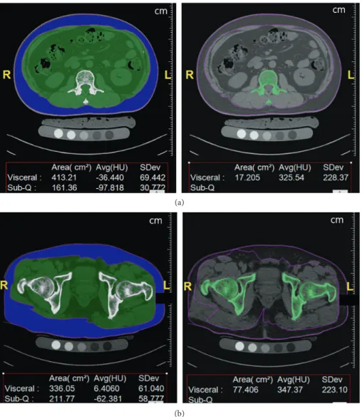
(a)
(b)
Figure 1: Screenshots of the semiautomatic calculation software (FatScan, N2 systems): (a) at the L2 level, the circumferences of the body and cross-sectional area of bone are segmented; and (b) at the hip level, the circumferences of the body and cross-sectional area of the bone
are segmented. In this case, the circumference of the L2 level is 89.559 cm, and the cross-sectional area of L2 is 17.205 cm2. The
commercial software Interactive Data Language (IDL) (Exelis Vis Inc., Boulder, CO, USA).
2.7. Comparison of Finite Element Analysis Results. This
study performed FE analysis to quantitatively investigate the effect of the estimated BMD on the structural behavior; the reference BMD was used as the ground truth. Segmentation of spine and hip images was first conducted using ITK-SNAP 3.6.0 [30]; hole filling and surface smoothing were implemented as postprocessing [31]. Then, each voxel in the segmented images was directly converted to a corresponding 8-node solid element. To assign the material properties required for the FE analysis, both the estimated and refer-ence BMD values of each voxel were converted into the elastic moduli of each finite element by using the BMD-modulus relationship for the spine [32] and the femur [33] as follows:
for the spine, E � 5124ρ1.7(MPa),
(3)
for the femur, E �6850ρ
1.49(MPa) if ρ ≤ 1.64 g·cm−3,
E �4293ρ2.39(MPa) if ρ > 1.64 g·cm−3,
(4) where E is Young’s modulus of each finite element and ρ denotes the BMD of each voxel. For comparison, the linear volume fraction approach, which has been widely used due to easy implementation in the literature [34–37], was also used to assign the elastic modulus of each element as follows:
E � E0×(BVF) (MPa), (5)
where (BVF) denotes the voxelwise volume fraction, which was linearly scaled to include the range of 0%–100% with the minimum and maximum values of voxel intensity for pure marrow and bone, respectively, in the CT images; E0 is the
maximum elastic modulus obtained by the reference BMD (10.2 GPa for the spine and 8.4 GPa for the femur in this paper). Poisson’s ratio was identically set to 0.3 for both the spine and femur. Pure compression and sideways falling conditions [33, 38] were selected as boundary conditions for the spine and femur, respectively. For the spine, a resultant force of 2,000 N was uniformly and vertically applied on the vertebral superior endplate. On the other hand, a vertical resultant force of 1000 N was applied in the distributed form towards the center of the femoral head. All FE analyses were conducted using the commercial software ANSYS 14.0.
3. Results
For the CT image of each patient, α and β were determined using the known mineral densities and corresponding HU values of the external phantom. After α and β in equation (1) were determined for the patient-specific calibration, the reference BMD values of the lumbar spine and hip for each patient were calculated using equation (1).
Through the univariate analyses, the HU value and circumference of the body were determined to be statistically
significant (p < 0.05) for the lumbar spine; only the HU value was statistically significant (p < 0.05) for the hip. Note that the bone area was determined not to be significant (p > 0.05) for both the lumbar spine and hip. Therefore, the phan-tomless HU-to-BMD conversion equations for the lumbar spine and hip were derived from the multiple linear re-gression models as follows:
(BMD)phantomless�0.848 ×(HU) + 0.148
×(circumference) − 7.4 for the lumbar spine,
(BMD)phantomless�0.784 ×(HU) + 16.6 for the hip,
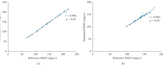
(6) where the units of BMD and circumference are mg/cc and cm, respectively. From Pearson’s correlation test (Figure 2), it was verified that the BMD values estimated using equation (6) were significantly correlated with the reference BMD values from equation (1). Pearson’s correlation coefficients were 0.998 and 0.984 for the lumbar spine and hip, re-spectively, and p < 0.05.
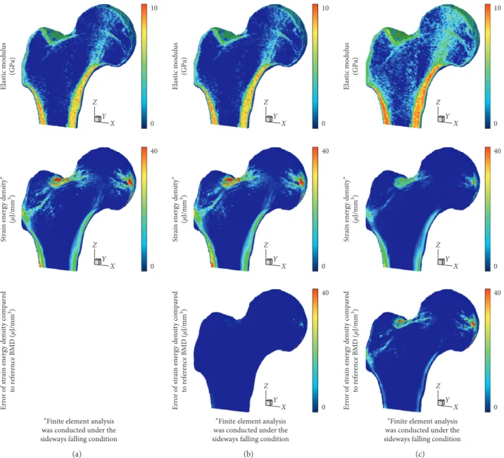
In terms of the voxelwise BMD, the proposed phan-tomless HU-to-BMD conversion equations gave values of 4.26 ± 0.60 mg/cc and 8.35 ± 0.57 mg/cc for RMSE of the BMD deviation for the lumbar spine and hip, respectively. Figures 3 and 4 indicate that the distributions of the elastic modulus obtained using the estimated BMD values (793 ± 1174 MPa and 1330 ± 1747 MPa for the spine and hip, respectively) are almost identical to those obtained using the reference BMDs (818 ± 1231 MPa and 1473 ± 2023 MPa for the spine and hip, respectively).
Therefore, the FEA with the estimated BMD values delivered the average strain energy densities of 2.04 μJ/mm3 and 0.08 μJ/mm3for the spine and hip, respectively, which are very close to those obtained with the reference BMDs (2.06 μJ/mm3for the spine and 0.08 μJ/mm3for the femur). In contrast, the elastic moduli estimated using the linear volume fraction approach (1756 ± 1492 MPa for the spine and 2146 ± 1967 MPa for the femur) were significantly higher than those obtained using the reference BMD values. Consequently, the average strain energy density for the linear volume fraction approach (0.51 μJ/mm3for the spine and 0.03 μJ/mm3for the femur) becomes much lower than that obtained using the reference BMD values. Note that total strain energy stored in the bone is inversely pro-portional to bone strength.
4. Discussion
BMD is a significant biomarker for bone strength [39] and therefore has an important function in the diagnostic criteria and therapeutic responses for osteoporosis. However, rou-tine CT scans (i.e., CT scans without a reference phantom) do not directly provide the BMD values of a target bone; rather, they provide the HU values. With the recent trend of FEA-based quantitative assessment, this study was prompted by the necessity for reliable phantomless HU-to-BMD conversion, which includes the effects of
patient-Reference BMD (mg/cc) Estima te d BMD (m g/cc) r = 0.998;p < 0.05 250 250 200 200 150 150 100 100 50 50 0 0 (a) Es tima te d BMD (m g/cc) Reference BMD (mg/cc) 200 200 150 150 100 100 50 50 0 0 r = 0.984; p < 0.05 (b)
Figure2: Pearson’s correlation test of the estimated BMD values and those derived using a reference phantom: (a) Pearson’s correlation
coefficient of 0.998 for the L2 level, and (b) Pearson’s correlation coefficient of 0.984 for the hip level (p< 0.05).
∗Finite element analysis was conducted under the pure
compression 8 0 50 0 Elastic modulus (GPa) Strain energy density ∗ (μ J/mm 3) Error of strain energy density compared to reference BM D (μ J/mm 3) Z Y X Z Y X (a)
∗Finite element analysis was conducted under the pure
compression 8 0 50 0 50 0 Elastic modulus (GPa) Strain energy density ∗ (μ J/mm 3) Error of strain energy density compared to reference BM D (μ J/mm 3) Z Y X Z Y X Z Y X (b)
∗Finite element analysis was conducted under the pure
compression 8 0 50 0 50 0 Elastic modulus (GPa) Strain energy density ∗ (μ J/mm 3) Error of strain energy density compared to reference BM D (μ J/mm 3) Z Y X Z Y X Z Y X (c)
Figure3: Distribution of elastic modulus, strain energy density, and error of strain energy density in the L2 vertebra: (a) case of using the
reference BMD values with an external phantom, (b) case of using BMD values estimated by the proposed phantomeless HU-to-BMD conversion, and (c) case of using the simplified conversion of linear volume fraction approach.
specific physical factors on the HU values. With 39 QCT images, the relationship between HU values and patient factors was investigated through multivariate analyses; linear regression models were obtained for phantomless HU-to-BMD conversion. A high positive correlation between the estimated and reference BMD values was found when using Pearson’s correlation tests. From these results, it was concluded that BMD values of the lumbar spine can be estimated in terms of HU values and circumferences but that BMD values of the hip can be calculated using only the HU values. This difference of applicable regression models between the lumbar spine and hip may stem from the different amounts of soft tissues and bone areas at the abdominal level and at the hip level. However, for typical HU values of bone (700 to 1500 HU) and waist circum-ferences (65.941 to 97.356 cm in this study), the influence of
waist circumference on the BMD is two orders of mag-nitude lower than that of HU. This implies that routine abdomen-pelvic or pelvic CT images (i.e., images obtained without using a reference phantom) have a high potential to be available for phantomless HU-to-BMD conversion through a process similar to the one proposed in this study. Recently, asynchronous calibration QCT has been in-troduced with excellent correlations, allowing for the quantification of BMD without the use of a calibration phantom [40, 41]. However, because the asynchronous phantomless QCT does not consider patient’ factors which can affect HU values, it showed poor repeatability [42]. It would be more reliable to combine patient factors (e.g., size and body composition) with phantomless QCT.
Figures 5 and 6 clearly show the similarity of the esti-mated and reference BMD values of each voxel. In terms of
10
0 40
0
∗Finite element analysis was conducted under the sideways falling condition
Elastic modulus
(GPa)
Strain energy density
∗
(μ
J/mm
3)
Error of strain energy density compared
to reference BMD ( μJ/mm 3) Z Y X Z Y X (a) 10 0 40 0 40 0 ∗Finite element analysis
was conducted under the sideways falling condition
Elastic modulus
(GPa)
Strain energy density
∗
(μ
J/mm
3)
Error of strain energy density compared
to reference BMD ( μJ/mm 3) Z Y X Z Y X Z Y X (b) 10 0 40 0 40 0 ∗Finite element analysis
was conducted under the sideways falling condition
Elastic modulus
(GPa)
Strain energy density
∗
(μ
J/mm
3)
Error of strain energy density compared
to reference BMD ( μJ/mm 3) Z Y X Z Y X Z Y X (c)
Figure4: Distribution of elastic modulus, strain energy density, and error of strain energy density in the proximal femur: (a) case of using
the reference BMD values with an external phantom, (b) case of using BMD values estimated by the proposed phantomeless HU-to-BMD conversion, and (c) case of using the simplified conversion of linear volume fraction approach.
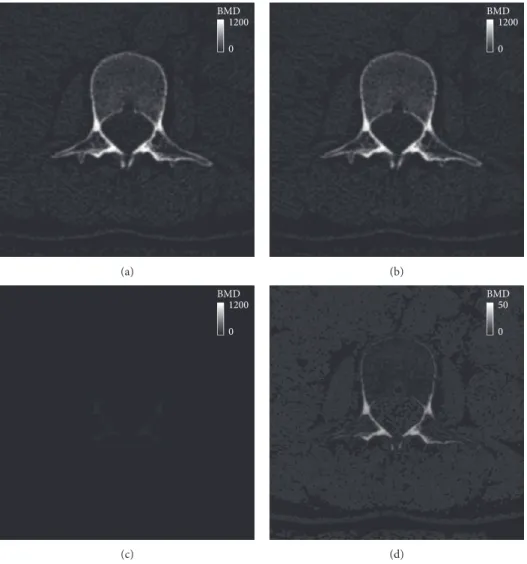
root-mean-square error (RMSE), the voxelwise BMD de-viation (4.26 ± 0.60 mg/cc for the lumbar spine and 8.35 ± 0.57 mg/cc for the hip in this study) can be regarded neg-ligible, compared with the maximum BMD (1000 mg/cc as shown in Figures 5(c) and 6(c)). Because an RMSE value can provide a representative value of the voxelwise BMD de-viation for a region of interest, it can be concluded that the proposed phantomless HU-to-BMD conversion equations precisely estimate voxelwise BMD values for the lumbar spine and hip, thereby providing a reliable spatial BMD distribution in 3D. It is interesting to note that, as clearly depicted in Figures 5(d) and 6(d), the errors of the BMD values estimated using the proposed equations are linearly proportional, albeit negligibly, to their BMD values. Note that, for clearer visualization, the maximum BMD in the legend in Figures 5(d) and 6(d) was set to be different from that in Figures 5(c) and 6(c). This linear proportionality of BMD conversion errors stems from the statistically pre-determined slope and y-intercept in equation (6), which are set in order to compensate for the patient-specific variation in attenuation.
As a more reliable tool for bone strength assessment [43], patient-specific FEA-based quantitative assessment requires voxelwise BMD data in order to assign the elastic modulus of each finite element through the BMD-modulus relationship. Patient-specific phantomless calibration of CT with an in-ternal phantom has been also recently proposed to apply to preexisting clinical CT for quantitative bone densitometry and bone strength assessment for diagnostic and monitoring purposes [44]. However, when voxelwise BMD data were unknown due to no QCT examination, many studies have assumed that the elastic modulus of each finite element is linearly proportional to the volume fraction of voxel in-tensity with a range of 0 to 1 (thus, a range between the minimum and maximum values for pure marrow and bone, respectively) [34–37]. This simplified approach can cause non-negligible errors in the FEA results, as clearly shown in Figures 3 and 4. Considering that the BMD-modulus re-lationship for the spine and femur, validated in the literature [45, 46], is typically nonlinear, a simplified linear pro-portionality (equation (5) in this paper) causes the in-termediate elastic moduli to become higher than those
BMD 1200 0 (a) BMD 1200 0 (b) BMD 1200 0 (c) BMD 50 0 (d)
Figure 5: BMD contour plot at the axial level of the L2 vertebra: (a) the reference BMD using an external phantom, (b) BMD estimated using the proposed phantomless HU-to-BMD conversion, (c) a deviation between the reference and estimated BMD values, and (d) BMD deviation on a different scale.
derived by the BMD-modulus relationship (equations (3) and (4) in this paper) when the maximum elastic moduli are set to be the same. Consequently, apparent bone stiffness becomes higher (i.e., lower total strain energies stored in Figures 3(c) and 4(c)) than it actually should be. In contrast, the voxelwise BMD values that were estimated using the proposed phantomless conversion led to reliable FEA re-sults, which were nearly identical to those obtained with the aid of QCT examination. These results demonstrate the potential of the proposed phantomless HU-to-BMD con-version to conduct reliable FEA-based quantitative assess-ment using routine CT images without the aid of QCT examination. Accurate voxelwise BMD estimation is also essential for the bone microstructure reconstruction approach recently proposed [47, 48].
The limitations of this study should be addressed. The proposed phantomless HU-to-BMD equation is based on the QCT protocol: 120 kVp, 150 effective mAs, 3 mm slice thickness, and B40s medium kernel. For better accessi-bility, the proposed formula should be extended to in-clude routine CT protocols. However, considering the
radiation dose modulation techniques, the simple equations of kVp or mAs might not be adequate. Fur-thermore, the influence of the increased density of the contrast media was not evaluated. Because the CT density depends on the phase after the contrast injection, phantomless BMD estimation should be undertaken carefully when using contrast-enhanced CT images. Fi-nally, although it has been reported that distinct CT scanners with the same acquisition protocol can have different scan data [49], this study used only a single kind of CT scanner due to a lack of availability. Therefore, the proposed method should be revisited more in depth for other kinds of CT scanners.
With follow-up research, the proposed models for phantomless HU-to-BMD conversion could be ex-tended to utilize routine CT images. Because routine CT scans are performed in daily practice, the proposed model would enable patients to avoid additional radi-ation exposure for BMD measurement. Furthermore, FEA-based quantitative assessment would be available for osteoporosis study of large populations, which can
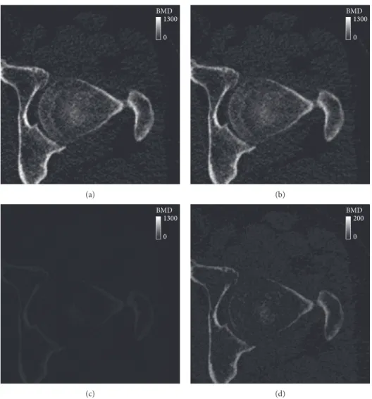
BMD 1300 0 (a) BMD 1300 0 (b) BMD 1300 0 (c) BMD 200 0 (d)
Figure 6: BMD contour plot at the axial level of the hip joint: (a) the reference BMD using an external phantom, (b) BMD estimated using the proposed phantomless HU-to-BMD conversion, (c) a deviation between the reference and estimated BMD values, and (d) BMD deviation on a different scale.
provide more reliable diagnostic data in translational medicine.
Data Availability
The QCT scan data used to support the findings of this study have not been made available because internal data research board does not permit data sharing without specific agreement.
Conflicts of Interest
The authors declare that they have no conflicts of interest regarding this work.
Acknowledgments
This work was partially supported by the National Research Foundation of Korea (NRF) grant funded by the Korea government (MSIP) (No. NRF-2017R1A2B4011760). This research was also partially supported by Basic Science Re-search Program through the National ReRe-search Foundation of Korea (NRF) funded by the Ministry of Education, Sci-ence and Technology (2012R1A1A2042165), South Korea.
References
[1] M. Iki, “[Epidemiology of bone and joint disease–the present and future. Epidemiology of osteoporosis and osteoporotic fracture in Japan],” Clinical Calcium, vol. 24, pp. 657–664, 2014.
[2] W. D. Leslie and S. N. Morin, “Osteoporosis epidemiology 2013,” Current Opinion in Rheumatology, vol. 26, no. 6, pp. 440–446, 2014.
[3] R. M. Pereira, J. E. Corrente, W. H. Chahade, and N. H. Yoshinari, “Evaluation by dual X-ray absorptiometry (DXA) of bone mineral density in children with juvenile chronic arthritis,” Clinical and Experimental Rheumatology, vol. 16, no. 4, pp. 495–501, 1998.
[4] G. M. Blake and I. Fogelman, “The role of DXA bone density scans in the diagnosis and treatment of osteoporosis,”
Post-graduate Medical Journal, vol. 83, no. 982, pp. 509–517, 2007.
[5] J. S. Finkelstein, A. Klibanski, and R. M. Neer, “Evaluation of lumber spine bone mineral density (BMD) using dual energy x-ray absorptiometry (DXA) in 21 young men with histories of constitutionally-delayed puberty,” Journal of Clinical
En-docrinology and Metabolism, vol. 84, no. 9, pp. 3403-3404,
1999.
[6] D. Marshall, O. Johnell, and H. Wedel, “Meta-analysis of how well measures of bone mineral density predict occurrence of osteoporotic fractures,” BMJ, vol. 312, no. 7041, pp. 1254– 1259, 1996.
[7] ACR–SPR–SSR practice guideline for the performance of quantitative computed tomography (QCT) bone densitometry. [8] E. M. Lewiecki, “Imaging technologies for assessment of skeletal health in men,” Current Osteoporosis Reports, vol. 11, no. 1, pp. 1–10, 2013.
[9] A. H. Habashy, X. Yan, J. K. Brown et al., “Estimation of bone mineral density in children from diagnostic CT images: a comparison of methods with and without an internal cali-bration standard,” Bone, vol. 48, no. 5, pp. 1087–1094, 2011. [10] J. E. Adams, “Quantitative computed tomography,” European
Journal of Radiology, vol. 71, no. 3, pp. 415–424, 2009.
[11] M. Ito, K. Hayashi, M. Yamada et al., “Relationship of osteophytes to bone mineral density and spinal fracture in men,” Radiology, vol. 189, no. 2, pp. 497–502, 1993. [12] N. Li, X. Li, L. Xu et al., “Comparison of QCT and DXA:
osteoporosis detection rates in postmenopausal women,”
International Journal of Endocrinology, vol. 2013, Article ID
895474, 5 pages, 2013.
[13] D. L. Kopperdahl, T. Aspelund, P. F. Hoffmann et al., “Assessment of incident spine and hip fractures in women and men using finite element analysis of CT scans,” Journal
of Bone and Mineral Research, vol. 29, no. 3, pp. 570–580,
2014.
[14] E. S. Orwoll, L. M. Marshall, C. M. Nielson et al., “Finite element analysis of the proximal femur and hip fracture risk in older men,” Journal of Bone and Mineral Research, vol. 24, pp. 475–483, 2009.
[15] J. Carballido-Gamio, R. Harnish, I. Saeed et al., “Structural patterns of the proximal femur in relation to age and hip fracture risk in women,” Bone, vol. 57, no. 1, pp. 290–299, 2013.
[16] J. H. Keyak, “Improved prediction of proximal femoral fracture load using nonlinear finite element models,” Medical
Engineering and Physics, vol. 23, no. 3, pp. 165–173, 2001.
[17] M. Bessho, I. Ohnishi, J. Matsuyama et al., “Prediction of strength and strain of the proximal femur by a CT-based finite element method,” Journal of Biomechanics, vol. 40, no. 8, pp. 1745–1753, 2007.
[18] J. H. Keyak and S. A. Rossi, “Prediction of femoral fracture load using finite element models: an examination of stress and strain based failure theories,” Journal of Biomechanics, vol. 33, no. 3, pp. 209–214, 2000.
[19] J. J. Schreiber, P. A. Anderson, H. G. Rosas et al., “Hounsfield units for assessing bone mineral density and strength: a tool for osteoporosis management,” Journal of Bone and Joint
Surgery-American Volume, vol. 93, no. 11, pp. 1057–1063,
2011.
[20] A. E. Papadakis, A. H. Karantanas, G. Papadokostakis et al., “Can abdominal multi-detector CT diagnose spinal osteo-porosis?,” European Radiology, vol. 19, no. 1, pp. 172–176, 2009.
[21] T. Baum, D. M¨uller, M. Dobritz et al., “Converted lumbar BMD values derived from sagittal reformations of contrast-enhanced MDCT predict incidental osteoporotic vertebral fractures,” Calcified Tissue International, vol. 90, no. 6, pp. 481–487, 2012.
[22] J. S. Bauer, T. D. Henning, D. M¨ueller et al., “Volumetric quantitative CT of the spine and hip derived from contrast-enhanced MDCT: conversion factors,” American Journal of
Roentgenology, vol. 188, no. 5, pp. 1294–1301, 2007.
[23] T. M. Link, B. B. Koppers, T. Licht et al., “In vitro and in vivo spiral CT to determine bone mineral density: initial experi-ence in patients at risk for osteoporosis,” Radiology, vol. 231, no. 3, pp. 805–811, 2004.
[24] R. M. Summers, N. Baecher, J. Yao et al., “Feasibility of si-multaneous computed tomographic colonography and fully automated bone mineral densitometry in a single examina-tion,” Journal of Computer Assisted Tomography, vol. 35, no. 2, pp. 212–216, 2011.
[25] J. G. Fletcher, C. D. Johnson, W. R. Krueger et al., “Contrast-enhanced CTcolonography in recurrent colorectal carcinoma: feasibility of simultaneous evaluation for metastatic disease, local recurrence, and metachronous neoplasia in colorectal carcinoma,” American Journal of Roentgenology, vol. 178, no. 2, pp. 283–290, 2002.
[26] T. Baum, D. M¨uller, M. Dobritz et al., “BMD measurements of the spine derived from sagittal reformations of contrast-enhanced MDCT without dedicated software,” European
Journal of Radiology, vol. 80, no. 2, pp. 140–145, 2011.
[27] B. J. Schwaiger, A. S. Gersing, T. Baum et al., “Bone mineral density values derived from routine lumbar spine multi-detector row CT predict osteoporotic vertebral fractures and screw loosening,” American Journal of Neuroradiology, vol. 35, no. 8, pp. 1628–1633, 2014.
[28] A. Barwick, J. Tessier, J. Mirow, X. J. de Jonge, and V. Chuter, “Computed tomography derived bone density measurement in the diabetic foot,” Journal of Foot and Ankle Research, vol. 10, no. 1, p. 11, 2017.
[29] A. Emami, H. Ghadiri, M. R. Ay et al., “A new phantom for performance evaluation of bone mineral densitometry using DEXA and QCT,” in Proceedings of IEEE Nuclear Science
Symposium Conference Record, pp. 3441–3445, Valencia,
Spain, October 2011.
[30] P. A. Yushkevich, J. Piven, H. C. Hazlett et al., “User-guided 3D active contour segmentation of anatomical structures: significantly improved efficiency and reliability,” Neuroimage, vol. 31, no. 3, pp. 1116–1128, 2006.
[31] J. J. Kim, J. Nam, and I. G. Jang, “Fully automated seg-mentation of a hip joint using the patient-specific optimal thresholding and watershed algorithm,” Computer Methods
and Programs in Biomedicine, vol. 154, pp. 161–171, 2017.
[32] J. Homminga, H. Weinans, W. Gowin et al., “Osteoporosis changes the amount of vertebral trabecular bone at risk of fracture but not the vertebral load distribution,” Spine, vol. 26, no. 14, pp. 1555–1561, 2001.
[33] E. Verhulp, B. van Rietbergen, and R. Huiskes, “Comparison of micro-level and continuum-level voxel models of the proximal femur,” Journal of Biomechanics, vol. 39, no. 16, pp. 2951–2957, 2006.
[34] S. N. Hwang, F. W. Wehrli, and J. L. Williams, “Probability-based structural parameters from three-dimensional nuclear magnetic resonance images as predictors of trabecular bone strength,” Medical Physics, vol. 24, no. 8, pp. 1255–1261, 1997. [35] C. S. Rajapakse, A. Hotca, B. T. Newman et al., “Patient-specific hip fracture strength assessment with microstructural MR imaging–based finite element modeling,” Radiology, vol. 283, no. 3, pp. 854–861, 2017.
[36] N. Zhang, J. F. Magland, C. S. Rajapakse et al., “Assessment of trabecular bone yield and post-yield behavior from high-resolution MRI-based nonlinear finite element analysis at the distal radius of premenopausal and postmenopausal women susceptible to osteoporosis,” Academic Radiology, vol. 20, no. 12, pp. 1584–1591, 2013.
[37] G. Chang, S. Honig, R. Brown et al., “Finite element analysis applied to 3-T MR imaging of proximal femur micro-architecture: lower bone strength in patients with fragility fractures compared with control subjects,” Radiology, vol. 272, no. 2, pp. 464–474, 2014.
[38] L. Cristofolini, M. Juszczyk, S. Martelli et al., “In vitro repli-cation of spontaneous fractures of the proximal human femur,”
Journal of Biomechanics, vol. 40, no. 13, pp. 2837–2845, 2007.
[39] L. Lenchik, R. Shi, T. C. Register et al., “Measurement of trabecular bone mineral density in the thoracic spine using cardiac gated quantitative computed tomography,” Journal of
Computer Assisted Tomography, vol. 28, no. 1, pp. 134–139,
2004.
[40] J. K. Brown, W. Timm, G. Bodeen et al., “Asynchronously calibrated quantitative bone densitometry,” Journal of Clinical
Densitometry, vol. 20, no. 2, pp. 216–225, 2017.
[41] L. Wang, Y. Su, Q. Wang et al., “Validation of asynchronous quantitative bone densitometry of the spine: accuracy, short-term reproducibility, and a comparison with conventional quantitative computed tomography,” Scientific Reports, vol. 7, no. 1, p. 6284, 2017.
[42] P. J. Pickhardt, L. J. Lee, A. M. del Rio et al., “Simultaneous screening for osteoporosis at CT colonography: bone mineral density assessment using MDCT attenuation techniques compared with the DXA reference standard,” Journal of Bone
and Mineral Research, vol. 26, no. 9, pp. 2194–2203, 2011.
[43] R. P. Crawford, C. E. Cann, and T. M. Keaveny, “Finite el-ement models predict in vitro vertebral body compressive strength better than quantitative computed tomography,”
Bone, vol. 33, no. 4, pp. 744–750, 2003.
[44] D. C. Lee, P. F. Hoffmann, D. L. Kopperdahl, and T. M. Keaveny, “Phantomless calibration of CT scans for measurement of BMD and bone strength-Inter-operator re-analysis precision,” Bone, vol. 103, pp. 325–333, 2017. [45] B. Helgason, E. Perilli, E. Schileo et al., “Mathematical
re-lationships between bone density and mechanical properties: a literature review,” Clinical Biomechanics, vol. 23, no. 2, pp. 135–146, 2008.
[46] N. K. Knowles, J. M. Reeves, and L. M. Ferreira, “Quantitative computed tomography (QCT) derived bone mineral density (BMD) in finite element studies: a review of the literature,”
Journal of Experimental Orthopaedics, vol. 3, no. 1, p. 36, 2016.
[47] J. J. Kim, J. Nam, and I. G. Jang, “Computational study of estimating 3D trabecular bone microstructure for the volume of interest from CT scan data,” International Journal for
Numerical Methods in Biomedical Engineering, vol. 34, no. 4,
article e2950, 2017.
[48] J. J. Kim and I. G. Jang, “Image resolution enhancement for healthy weight-bearing bones based on topology optimiza-tion,” Journal of Biomechanics, vol. 49, no. 13, pp. 3035–3040, 2016.
[49] L. Balkay, A. Oszl´anszki, and A. K. Krizs´an, “Comparison of patient doses at different CT scanners with same acquisition protocol,” in Proceedings of IEEE Nuclear Science Symposium
and Medical Imaging Conference Record (NSS/MIC),
Stem Cells
International
Hindawi www.hindawi.com Volume 2018 Hindawi www.hindawi.com Volume 2018 INFLAMMATIONEndocrinology
International Journal ofHindawi www.hindawi.com Volume 2018 Hindawi www.hindawi.com Volume 2018
Disease Markers
Hindawi www.hindawi.com Volume 2018 BioMed Research InternationalOncology
Journal of Hindawi www.hindawi.com Volume 2013 Hindawi www.hindawi.com Volume 2018Oxidative Medicine and Cellular Longevity
Hindawi
www.hindawi.com Volume 2018
PPAR Research
Hindawi Publishing Corporation
http://www.hindawi.com Volume 2013 Hindawi www.hindawi.com
The Scientific
World Journal
Volume 2018 Immunology Research Hindawi www.hindawi.com Volume 2018 Journal ofObesity
Journal of Hindawi www.hindawi.com Volume 2018 Hindawi www.hindawi.com Volume 2018 Computational and Mathematical Methods in Medicine Hindawi www.hindawi.com Volume 2018Behavioural
Neurology
Ophthalmology
Journal of Hindawi www.hindawi.com Volume 2018Diabetes Research
Journal ofHindawi
www.hindawi.com Volume 2018
Hindawi
www.hindawi.com Volume 2018
Research and Treatment
AIDS
Hindawi
www.hindawi.com Volume 2018
Gastroenterology Research and Practice
Hindawi www.hindawi.com Volume 2018