Generalization of the Fourier Convergence Analysis in the Neutron Diffusion Eigenvalue Problem

(1)

Generalization of the Fourier Convergence Analysis in the Neutron Diffusion Eigenvalue Problem

Hyun Chul Lee, Jae Man Noh, Hyung Kook Joo

Korea Atomic Energy Research Institute, 150 Deokjin-Dong, Yuseong-Gu, Daejeon, Korea, lhc@kaeri.re.kr

1. Introduction

Fourier error analysis has been a standard technique for the stability and convergence analysis of linear and nonlinear iterative methods. Lee et al proposed new 2-D/1-D coupling methods and demonstrated several advantages of the new methods by performing a Fourier convergence analysis of the methods as well as two existing methods for a fixed source problem[1].

We demonstrated the Fourier convergence analysis of one of the 2-D/1-D coupling methods applied to a neutron diffusion eigenvalue problem[2]. However, the technique in Ref. 2 cannot be used directly to analyze the convergence of the other 2-D/1-D coupling methods since some algorithm-specific features were used in our previous study.

In this paper we generalized the Fourier convergence analysis technique proposed in Ref. 2 and analyzed the convergence of the 2-D/1-D coupling methods applied to a neutron diffusion eigenvalue problem using the generalized technique.

2. Methods and Results

The 2-D/1-D coupling methods described in Ref. 1 can be directly applied to eigenvalue problems. They begin with the axially averaged 2-D diffusion equation which can be written for each plane as in Eq. (1),

(

zk zk

)

zk eff k k f k k k k k h J J k y D y x D x , , 1 , , − − Σ = Σ +       ∂ ∂ ∂ ∂ + ∂ ∂ ∂ ∂ − +

φ

ν

φ

, (1)

and the radially averaged 1-D diffusion equation for each axial mesh which can be written as in Eq. (2),

(

)

(

)

( , ) ( , ) ( , ) ( , ) ,( , ) ( , ) , 1 , , 1 , i j i j i j i j f i j i j eff x i x i x y j y j y D k z z J J h J J h

φ

ν

φ

+ + ∂ ∂ − + Σ = Σ ∂ ∂ − − − − . (2)

Method A in Ref. 1 is to evaluate the TL of the 2-D/1-D equations directly from the 1-D/2-D solutions. The effective multiplication factor can be updated by applying the power iteration as follow :

(

)

( )n (n1) ( )n (n1)

eff eff f f

V V

k =k −

∫

w

ν φ

Σ dV

∫

w

ν φ

Σ − dV , (3)

where

w

is an arbitrary weighting function.

The model problem in Ref. 2 was used to analyze the convergence of method A applied to an eigenvalue problem. The model problem is a 3-D one-group diffusion

eigenvalue problem in a homogeneous finite multiplying medium of N planes with periodic boundary conditions. It is obvious that the exact solution to the model problem is

0 φ

φ = and keff =k∞=νΣf Σ. Two basic assumptions are introduced in order to simplify the convergence analysis. These are (1) solving the 2-D problems plane by plane, which means solving them iteratively in the z-direction and (2) solving the 2-D problem by a direct inversion of the 2-D operator in a given plane. The second assumption leads to a zero radial leakage during the iterations, and simplifies Eqs (1) and (2) to:

(

J J

)

h keff zk zk k k = Σ − , 1− , Σ

φ

ν

φ

+ , (4a) ) , ( ) , ( ) , ( 1 j i eff j i j i k z D z ∂

φ

+Σ

φ

=

ν

Σ

φ

∂ ∂ ∂ −

.

(4b)

The iterative algorithm of method A applied to the eigenvalue problem with one inner iteration per outer iteration can be expressed by the following equations :

(

( 1)

)

, ) 1 ( 1 , ) 1 ( ) 1 ( ) ( 1 1 − − + − − Σ − − = Σ n k z n k z n k f n eff n k J J h k

ν

φ

, (5a)

∑

− − = ' ) 1 ( ' ' ) ( ' ) 1 ( ) ( k n k k n k n eff n eff k k

φ

, (5b)

(

( )

)

1 ) ( ) ( ) ( , n k n k n n k z A J =−

φ

−

φ

₋ , (5c) where

( )

[

]

D k h h D A n eff f n n n n ) ( ) ( ) ( 2 2 ) ( ) ( ; 2 / sinh 4 Σ − Σ = =

κ

ν

κ

Note that the two-node analytic nodal method was used to solve the axial 1-D equation and also that a constant weighting function was used to get Eq. (5b).

As we did in the fixed source problem, let’s introduce a first order perturbation of ( )n

k φ , (n) eff k , and (n) A in Eq. (5).

(

( )

)

0 ) (

₁

n k n k

φ

εξ

φ

=

+

, (6a)

(

)

(

)

( ) ( ) 1keffn = 1k∞ 1+

εδ

n , (6b)

(

( )

)

0 ) ( 1 n n A A = +

εθ

, (6c) where ( ) ( ) 0 n eff n k k A Lim A D h ∞ → = = .

Note that _δ( n) _and_θ(n) _{as well as} ( n) eff

k and A(n) are independent of the mesh index k.

Inserting Eq. (6) into Eq. (5) and dropping the

( )

_ε

2 O

terms yields the following linearized equation :

(

)

( ) ( 1) ( 1) 2 2 ( 1) ( 1) ( 1) 1 2 1 n n n n n n k k L h k k k ξ δ − ξ − ξ − ξ − ξ − − + = + + − + , (7a)

Transactions of the Korean Nuclear Society Autumn Meeting Busan, Korea, October 27-28, 2005

(2)

∑

− = − − − = + = + 1 0 ' ) 1 ( ' ) 1 ( 1 0 ' ) ( ' ) ( 1 1 N k n k n N k n k n N N

ξ

δ

ξ

δ

. (7b)

Note that _{θ disappeared in the linearized equation.}( n) There are only N independent bases for the flux vector because the dimension of the flux vector is N . We can choose the N eigenvectors from the lowest mode as the basis. The flux can be expanded by the N

eigenvectors, _eiλmx

(

)

1 , , 1 , 0 − = N m Λ , corresponding to the

eigenmodes λ_m=2mπ

( )

Nh which satisfy the periodic boundary conditions of the model problem. Therefore, we can introduce the following Fourier ansatz :

h k i n m m n m k n k m e a ( 1/2) ) ( , ) ( ₌

_ξ

₌

_ω

λ +

ξ

, (8a) n n b ₀ ) (

_ω

δ

= , (8b) Note that only some discrete values of the wave number,

m

λ , are allowed in Eq. (8) whereas a continuous wave number is allowed in the fixed source problem. Among the eigenmodes, λ0=0 forms the fundamental

mode solution of the flux, ()

0 ,

1+ξkn for the model problem, and the other modes, λ_m

(

m=1,2,Λ,N−1

)

, form the higher mode error term of the flux, ()

, n m k

ξ . As indicated above, _{δ is independent of the space, which means that}(n) only λ0=0 is allowed for the wave number of the Fourier ansatz of _{δ .}(n)

It is trivial to show that

(

1,2, , 1

)

0 1 0 ' ) ( ,' = = −

∑

− = N m N k n m k Λ

ξ

. (9)

Using Eq. (9), we can simply Eq. (7) for m>0 :

(

)(

)

( ) ( 1) 2 2 ( 1) ( 1) ( 1) , , 1, 2 , 1, n n n n n k m k m L h k m k m k m

ξ

−

ξ

−

ξ

−

ξ

− − + = + − + . (10)

We can also simplify Eq. (7) for m=0 :

) 1 ( 0 *, ) 1 ( ) ( 0 *, − − ₊ = n n n

_δ

_ξ

ξ

, (11a) ) 1 ( 0 *, ) 1 ( ) ( 0 *, ) (n ₊

_ξ

n ₌

_δ

n− ₊

_ξ

n−

δ

, (11b) where n n k n a0 0 ) ( 0 , ) ( 0 *,

ξ

ω

ξ

= = .

From Eq. (10) and (11), we get

0 0 =

ω

, (12a)

(

2 2

)

( )

(

)

1 2 cos 1 0 m L h m m

ω

= + _

τ

− _ > . (12b)

Note that τ =_m λ_mh are 2π N, 4π N,Λ , 2

(

N−1

)

π N . The spectral radius of the linearized algorithm of method A for the eigenvalue problem is given by :

m N m

ω

ρ

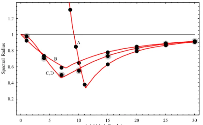
Max 1 , , 1 , 0 − = = Λ . (13)

One can directly apply the Fourier convergence analysis demonstrated above to the other 2-D/1-D coupling methods. Figure 1 shows the spectral radius of the 2-D/1-D coupling methods as a function of the axial mesh size for the model problem with N =4 , D=0.833333 ,

0.02

Σ = , and νΣf =0.019 . The line is the analytic

spectral radius obtained by the Fourier analysis and the dots are the numerical ones. The large gray dots are used for method D to distinguish them from those for method C. As indicated, a good agreement is observed between the analytic and numerical results. As we expected, we got the same result as that in Ref. 2 for method A. Though method A is the best in terms of a spectral radius for a large mesh size, it diverges for a small mesh size. The other methods are always stable regardless of the axial mesh size. The spectral radius of methods C and D are smaller than that of method B in the range of a practical mesh size. The spectral radius of methods C and D are identical while that of D is smaller than that of C in a fixed source problem[1]. It is interesting that the spectral radius in the eigenvalue problem approaches 1 as the mesh size increases while it approaches zero in the fixed source problem.

0 5 10 15 20 25 30

Axial Mesh Size h in cm 0.2 0.4 0.6 0.8 1 1.2 la rt ce p S s ui da R A B C,D

Figure 1. The spectral radius of 2-D/1-D coupling methods 3. Conclusion

In this paper we generalized the Fourier convergence analysis technique proposed in Ref. 2 and analyzed the convergence of the 2-D/1-D coupling methods applied to a neutron diffusion eigenvalue problem using the generalized technique. The analysis showed that the newly proposed methods, C and D, are better than the existing methods, A and B, even for the eigenvalue problems.

REFERENCES

[1] H. C. Lee, D. Lee, and T. J. Downar, “Iterative Two- and One-Dimensional Methods for Three-Dimensional Neutron Diffusion Calculations,” Nucl. Sci. Eng., 151, 46-54 (2005)

[2] H. C. Lee, J. M. Noh, H. K. Joo, “Fourier Convergence Analysis Applied to Neutron Diffusion Eigenvalue Problem,” Proceedings of the Korean Nucl. Soc. Autumn Meeting, Yongpyong, Korea, October 2004. Korean Nucl. Soc. (2004)