The Economic Effect of the
Basic Pension and National
Health Insurance
- A Social Accounting Matrix Approach
Jongwook Won, Senior Research Fellow ⓒ 2016
Korea Institute for Health and Social Affairs
All rights reserved. No Part of this book may be reproduced in any form without permission in writing from the publisher
Korea Institute for Health and Social Affairs Building D, 370 Sicheong-daero, Sejong city 30147 KOREA
http://www.kihasa.re.kr
Ⅰ. Introduction ···1
Ⅱ. Methodology of Analysis ···7
1. Social Accounting Matrix (SAM) ···9
2. Creating a macro SAM ···10
3. Creating bridge matrices for micro SAMs ···11
4. Creating micro SAMs ···16
5. Creating multiplier matrices ···18
Ⅲ. Basic Pension (BP) ···21
1. Underlying assumptions: fiscal streamlining and tax financing ···23
2. Economic ripple effects of fiscal streamlining ···27
3. Economic ripple effects of tax financing ···28
4. Income redistribution effect of the BP ···32
5. Conclusion ···33
Ⅳ. National Health Insurance (NHI) ···35
1. Scenarios for analysis ···37
5. Conclusion ···56
List of Tables
<Table 1> Structure of Macro SAM ···10 <Table 2> Bridge Matrix ···11 <Table 3> Separation of Production Activities and Commodities
Account ···12 <Table 4> Micro Breakdown of the Household Sector ···13 <Table 5> Types of Assets in the Micro Breakdown of the Household
Revenue Vector ···13 <Table 6> Bridge Matrix for Household Revenue Vector ···14 <Table 7> Items in Household Sectors Other Than Household
Consumption ···15 <Table 8> Bridge Matrix of Sectors Except Household Consumption · 15 <Table 9> Fiscal Streamlining: Reducing Government Spending on
Other Sectors ···24 <Table 10> Additional Tax Burden for the BP: Increasing Income Taxes ···26 <Table 11> BP Payout Scenarios ···27 <Table 12> Production-Inducing Effects of Tax Financing for the BP 29 <Table 13> Production-Inducing Effects of Tax Financing (Increasing
Income Taxes) and BP Payouts on 32 Industries ···29 <Table 14> Income-Generating Effects of Tax Financing for the BP ···30 <Table 15> Income-Generating Effects of Tax Financing (Increasing
Income Taxes) and BP Payouts on 32 Industries ···31 <Table 16> Gini Coefficients Before and After BP Payouts ···32 <Table 17> NHI Spending Scenarios for SAM Analysis ···38 <Table 18> NHI Expenditures and Revenue by Year (2009 to 2013) ····38
Increasing NHI by 10 Percent ···45 <Table 21> Industry-by-Industry Production-Inducing Effect of
Increasing NHI by 10 Percent (Omitted) ···47 <Table 22> Production-Inducing Effect of Increasing NHI Expenditure
by BP Budget ···50 <Table 23> Comparison of Production-Inducing Effects of the BP and
NHI (Increased by Same Amount) ···50 <Table 24> Production-Inducing Effect by Industry When NHI
Expenditure Is Increased (by BP Budget of 2015) ···52 <Table 25> Production-Inducing Effect by Industry When NHI Expenditure Is Increased (by BP Budget of 2015) (Omitted) ···54
List of Figures
〔Figure 1〕 SAM Construction Flow Chart ···16 〔Figure 2〕 Process of Creating Micro SAMs: Household Revenue Taxes ···17 〔Figure 3〕 Macro and Micro SAMs ···17 〔Figure 4〕 NHI Expenditure and BP Projections (until 2050) ···39
Korea’s Basic Old Age Pension was replaced with the Basic Pension in July 2014, but the old-age poverty rate remains high and much of the population does not benefit from the National Pension. Korea may have achieved astonishing economic growth over the last few decades, but its old-age poverty rate (48.6 percent in 2011) far exceeds the OECD average of 10.9 percent. The Basic Pension, moreover, remains unlinked with other old-age protection schemes such as the National Pension, which, still in its early stages, has large coverage gaps and provides only a modest income replacement rate. It is thus critical to keep track of, and analyze the income protection ef-fect of the Basic Pension and the economic efef-fect of increasing Basic Pension benefits in order to increase the fiscal sustain-ability of the basic pension system and alleviate old-age poverty.
Based on our recognition of these issues, we analyze, in Chapter III, how the payout of basic pension benefits to elderly households would serve to increase the outputs of various sec-tors and industries and contribute to increasing incomes for all groups and classes across the economy. The assumptions un-derlying our analysis are that: (a) elderly households will spend
their pension income in a manner characteristic of elderly citi-zens, and (b) the old-age pension will help reduce income in-equality among elderly households. Our objective is to analyze and verify, in an objective and empirical manner, how the basic pension would improve the standard of living for the elderly and thereby contribute to the national economy at large.
Before proceeding with our analysis, we need first to discuss briefly the methodology of the Social Accounting Matrix (SAM). We use the SAM to estimate and measure the production-in-ducing and income-generating effects of the basic old-age pension on the national economy, as well as how the pension redistributes income, as measured by the Gini coefficient. Our analysis provides basic information with which policymakers can estimate the micro-level impact of the basic pension policy on old-age poverty.
The National Health Insurance (NHI) scheme is one of the four major social insurances in Korea, and claims, by far, the most government spending of all social insurances (KRW 53 trillion as of 2015). According to the Social Security Fiscal Projections of March 2015, NHI spending is expected to grow rapidly to reach between KRW 694 trillion and KRW 1,099 tril-lion by 2050. Such rapid growth of NHI spending calls for anal-yses of the NHI policy effects and measures to ensure their fis-cal sustainability. However, the need to find a proper method-ology for gauging and analyzing the policy effects of the NHI is
more urgent. In an attempt to go beyond the simplistic cost-ef-fect analysis of the NHI, we apply the SAM in this study to ana-lyze the micro- and macro-level ripple effects of the NHI on the rest of the national economy. More specifically, we focus on identifying the production-inducing effect of households’ health insurance spending on hospitals and other providers of medical care and services.
To this end, in Chapter IV, we survey the current status of the NHI in Korea. Afterward, we analyze the economic effects of increasing NHI spending on production and income.
Ⅱ
1. Social Accounting Matrix (SAM) 2. Creating a macro SAM
1. Social Accounting Matrix (SAM)
In this study, we use the SAM methodology to analyze the so-cioeconomic effect of the Basic Pension (BP) and National Health Insurance (NHI). The SAM, often understood as an ex-panded version of the input-output tables, is created by com-bining the data from the input-output tables and the National Accounts. SAMs are used to indicate the relationship between the value added and expenditures of a given country or region (Ko et al., 2014, 100). Generally, depending on the purpose of the research, macro SAMs can be multiplied by bridge matrices in order to divide accounts at the micro-level. The result is called the Micro Social Accounting Matrix, which conveys quantitative information on transactions between groups (Ko et al., 2014, 100). Bridge matrices based on raw micro-data have various applications. The resulting SAM clarifies the correla-tions between revenue and expenditure in various sectors of a given society and economy (Ko et al., 2014, 100).
1) The brief overview of the SAM methodology provided in this section is intended to facilitate the reader’s understanding, and consists mainly of excerpts from Chapter 4, Section 1, of Ko et al. (2014).
2. Creating a macro SAM
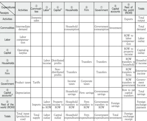
Table 1 shows an example of a macro SAM. It consists of cor-relations between revenue and expenditure across nine items, including production activities, commodities, and labor (Ko et al., 2014, 158-189).
<Table 1> Structure of Macro SAM
Expenditures Receipts Activities ② Commodi-ties ③
Labor1) Capital④ 1) Households⑤ Firm⑥ Government⑦
⑧ Capital accounts ⑨ Rest of the world (ROW) Totals
Activities Domestic sales Exports outputTotal
Commodities Intermediate demand consumptionHousehold consumption InvestmentGovernment demandTotal
Labor compensa-Labor tion ROW to labor compensa-tion Labor outlay ④
Capital Operating surplus
ROW to property income Capital outlay ⑤
Households incomeLabor Distributed profits Transfers Transfers
ROW transfers to household Househol d income ⑥ Firm Non-distributed
profits Transfers Transfers
ROW transfers to firms Enterprise income ⑦
Government Product taxes Tariffs Income taxes Corporate taxes
ROW transfers to government Govern-ment Income ⑧ Capital accounts2) Depreciation Household
savings Firm savings Government savings
Row to net capital transfers Total savings ⑨ Rest of the
world (ROW) Imports Labor income to ROW Property income to ROW Household transfers to ROW Firm transfers to ROW Government transfers to ROW Foreign savings Foreign exchange payment
Totals (production Total input cost)
Total
supply outlayLabor Capital outlay expendituresHousehold expendituresFirm expendituresGovernment investmentTotal Foreign exchange
receipt
3. Creating bridge matrices for micro SAMs
In order to create a micro SAM using the control total of a macro SAM, we need a bridge matrix that connects the two ma-trices (Ko et al., 2014, 174).
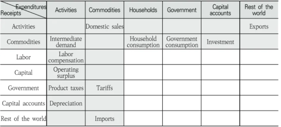
Table 2 provides an example of diverse bridge matrices that can be created. If our goal is to analyze the distribution of in-come by inin-come quintile, we need information on the inin-come transfers among economic actors, which is not found in the put-output tables alone. We thus need to insert the data on in-come transfers as a separate bridge matrix (Ko et al., 2014, 174).
<Table 2> Bridge Matrix
Expenditures
Receipts Activities Commodities Households Government accountsCapital Rest of the world
Activities Domestic sales Exports
Commodities Intermediate demand consumptionHousehold consumptionGovernment Investment Labor compensationLabor
Capital Operating surplus
Government Product taxes Tariffs Capital accounts Depreciation
Rest of the world Imports
<Table 3> Separation of Production Activities and Commodities Account
1. Agriculture, forestry and
fishery products 12. Electronic and electrical equipment 23. Finance and insurance services 2. Mining and quarrying
products 13. Precision instruments 24. Real estate and leasing 3. Food and beverages 14. Transportation equipment 25. Professional, scientific, and technological services 4. Textile and leather
products 15. Other manufactured and toll processed goods 26. Business support services 5. Wood, paper, and
printing 16. Electricity, gas, and steam 27. Public administration and national defense 6. Petroleum and coal
products 17. Water supply, waste, and recycling services 28. Education services 7. Chemical products 18. Construction 29. Medicine and healthcare 8. Non-metallic mineral
products 19. Wholesale and retail services 30. Social insurance services 9. Basic metal products 20. Transportation services 31. Social welfare services 10. Fabricated metal
products 21. Restaurant and accommodation services 32. Culture and other services 11. Machinery and equipment 22. Information, communications, and broadcasting services Source: Ko et al. (2014), 177.
For household-sector items in the macro SAM that needed to be broken down into micro-level items, we used the raw mi-cro-data of the Survey of Household Finances and Living Conditions (SHFLC) and Household Surveys (HS) to divide households into two groups (i.e., elderly and non-elderly), and further divide each group of households into 10 income deciles.
<Table 4> Micro Breakdown of the Household Sector
Exp.
Rev. Labor Capital Households Firm Government Rest of the world Commodities Household
consumption Households Labor
income
Distributed
profits Transfers Transfers
ROW transfers to household Firm Transfers Government Income taxes Capital accounts Household savings Rest of the world
Household transfers to
ROW
Source: Ko et al. (2014), 178.
Household revenue is broken down according to the system of categories used in the SHFLC, while household expenditure is categorized according to the system used in the HS.
“Assets” represent the sum of “financial”, “real”, and “other real” assets included in the raw micro-data of the 2014 SHFLC. The specific assets included under each of the three asset types are listed in Table 5 below.
<Table 5> Types of Assets in the Micro Breakdown of the Household Revenue Vector
Item Financial assets Real assets Other real assets
Household assets
Savings deposits, installment savings (savings with free deposits and withdrawals, installment savings funds, savings and guaranteed-cost insurance policies), deposit savings and funds, stocks and bonds, premiums, other savings, lease deposits on current housing
One’s home (detached houses, apartment units, row housing, household units in multi-household buildings, etc.), real estate other than one’s home, lease deposits and intermediate payments on mortgages or house prices.
Cars and other assets (facilities and inventories of business owners, construction and farming equipment, animals and plants, golf memberships, resort memberships, jewelry, antiques and artworks, expensive durables, intellectual property rights, etc.)
<Table 6> Bridge Matrix for Household Revenue Vector
Income distribution by household type and asset type
Wages (earned income) à assets Shared profits (property income) Business-to-household transfers (non-current income) Government -to-household transfers (transfer income) Overseas-to-household current transfers (annual income) ⑤ Households Elderly households 1st decile 0.0042 0.0035 0.0073 0.0014 0.0009 2nd decile 0.009 0.0064 0.0099 0.0063 0.0085 3rd decile 0.0159 0.0015 0.0107 0.0008 0.0142 4th decile 0.0241 0.0176 0.0099 0.0016 0.019 5th decile 0.0279 0.0145 0.017 0.0049 0.0233 6th decile 0.034 0.0204 0.0216 0.0108 0.0276 7th decile 0.0416 0.0409 0.0258 0.0106 0.0328 8th decile 0.0516 0.0238 0.0237 0.0237 0.039 9th decile 0.0639 0.0324 0.0344 0.0299 0.0482 10th decile 0.0991 0.0834 0.11 0.0482 0.0737 Non-elderly Households 1st decile 0.0129 0.0114 0.0294 0.0068 0.0093 2nd decile 0.0246 0.023 0.0338 0.0254 0.0229 3rd decile 0.0292 0.0219 0.0352 0.0229 0.0431 4th decile 0.0448 0.057 0.0439 0.0663 0.0519 5th decile 0.051 0.0681 0.0559 0.0905 0.0605 6th decile 0.0596 0.063 0.0637 0.1034 0.0772 7th decile 0.0702 0.0987 0.0759 0.1117 0.0866 8th decile 0.0842 0.0783 0.0723 0.1365 0.0977 9th decile 0.1015 0.103 0.1055 0.1211 0.1144 10th decile 0.1507 0.2312 0.2141 0.1772 0.1492 Total 1 1 1 1 1
<Table 7> Items in Household Sectors Other Than Household Consumption
Household-to-business transfers (non-consumption
expenditure)
Income taxes
(annual income) Household savings (savings amount)
Private transfers overseas (household expenditure)
Items
Annual loan interest and payments, secured loans (balances), lease deposits, securities investments, repaid debts, business capital, wedding capital, medical expenses, education expenses, living expenses, savings deposits/insurance policies held as loan securities
Income taxes
Installment savings (savings with free deposits and
withdrawals, installment savings funds, savings and guaranteed-cost insurance policies), deposit savings (savings and funds), stocks and bonds, and others (futures and options)
Private transfer income
Source: Won and Chang (2015), 13.
<Table 8> Bridge Matrix of Sectors Except Household Consumption
Note: The columns and rows have been modified for ease of writing. Source: Won and Chang
Expenditure item Asset type Household-to -business transfers (non-consumption expenditure) Income taxes (current income) Household savings (savings amount) Private transfers overseas (household expenditure) ⑤ Households Elderly households 1st decile 0.0003 0.0000 0.0017 0.0002 2nd decile 0.0055 0.0003 0.0049 0.0063 3rd decile 0.0102 0.0012 0.0084 0.0122 4th decile 0.0159 0.0025 0.0156 0.0173 5th decile 0.0222 0.0042 0.024 0.0213 6th decile 0.0251 0.0061 0.0328 0.0251 7th decile 0.0321 0.0088 0.0429 0.03 8th decile 0.0431 0.0135 0.0576 0.0362 9th decile 0.054 0.0219 0.0813 0.0441 10th decile 0.0916 0.0727 0.1154 0.064 Non-elderly households 1st decile 0.0254 0.0005 0.0027 0.0067 2nd decile 0.0333 0.0088 0.0079 0.0152 3rd decile 0.0404 0.0197 0.0134 0.0235 4th decile 0.0488 0.0319 0.025 0.054 5th decile 0.0583 0.0439 0.0384 0.0856 6th decile 0.0626 0.0595 0.0524 0.0909 7th decile 0.0732 0.0792 0.0686 0.0978 8th decile 0.0896 0.1048 0.0921 0.1065 9th decile 0.106 0.1508 0.13 0.1175 10th decile 0.1623 0.37 0.1847 0.1454 Total 1 1 1 1
4. Creating micro SAMs
For our analysis, we created a SAM with 90 columns and 90 rows, with the household revenue and consumption items in-cluded in the bridge matrix (Won and Chang, 2015, 13).
〔Figure 1〕 SAM Construction Flow Chart
〔Figure 2〕 Process of Creating Micro SAMs: Household Revenue Taxes
Source: Won and Chang
〔Figure 3〕 Macro and Micro SAMs
Source: Won and Chang
5. Creating multiplier matrices
The purpose of this study is to analyze the production-induc-ing and income-generatproduction-induc-ing effects of the BP and NHI, a task that requires the creation of multiplier matrices. Multiplier ma-trices indicate the quantitative ripple effects of exogenous changes. The creation of these matrices thus requires the iden-tification of endogenous and exogenous variables (Ko et al., 2014, 109).
A multiplier analysis of the effect of the BP and NHI reveals only the quantitative, fragmentary, and fixed aspects of the rip-ple effects, rather than providing an in-depth explanation as to why such effects would occur (Ko et al., 2014, 109). The analy-sis, however, is capable of showing the ripple effects of changes in social security expenditure on all industries of a given economy. A multiplier matrix consists of the following.
If we divide an n-number of endogenous accounts into three categories, i.e., production factors, institutions, and pro-duction, we may express the multiplier matrix of our SAM, , using as follows (Ko et al., 2014, 110).
As Equation 3-1 shows, we may express the endogenous ac-counts as the average expenditure tendency matrix of each sector and each input unit, and convert them into the multi-plier matrix of the SAM. Here, represents the total sum of all exogenous expenditures.
……… (1)
Where,
: endogenous accounts, : partition matrix indicating the “average expenditure tendency” of each sector, : unit input
Here, the total income effect is expressed as ,
which indicates how each change in the exogenous inputs would affect the endogenous variables (Ko et al., 2014, 112).
Ⅲ
1. Underlying assumptions: fiscal streamlining and tax financing
2. Economic ripple effects of fiscal streamlining 3. Economic ripple effects of tax financing 4. Income redistribution effect of the BP 5. Conclusion
1. Underlying assumptions: fiscal streamlining and
tax financing
A. Financing the BP through fiscal streamlining
We posited two different scenarios for the financing of the BP in the future. The first scenario involves fiscal streamlining —namely, reducing government spending on other programs and policies in order to finance the BP. The rates for the de-creases in government spending on other programs and poli-cies were obtained in reference to the government spending rates used for each sector in the micro SAMs (Won and Chang, 2015, 14).
2) For more details on the background of our analysis, the current status of the BP, the findings of the fiscal streamlining analysis, and the income redistribution effect of the pension, see Won and Chang (2015).
<Table 9> Fiscal Streamlining: Reducing Government Spending on Other Sectors
(Units: KRW 1 million, %)
B. Tax financing for the BP
The second scenario involves increasing taxes to finance the BP. In this scenario, households would reduce their ex-penditure on and consumption of commodities while paying higher income taxes (household-to-government transfers). We
Sector Government spending Proportion of government spending by industry Margin of decrease in funding for BP Balance of government spending for BP 49. Water supply, waste, and
recycling services 683,147 0.37 37,636.63 645,510.37
50. Construction 0 0.00 0.00 0.00
51. Wholesale and retail services 0 0.00 0.00 0.00 52. Transportation services 0 0.00 0.00 0.00 53. Restaurant and
accommodation services 1,698,040 0.93 93,550.14 1,604,489.86 54. Information, communications,
and broadcasting services 0 0.00 0.00 0.00 55. Finance and insurance
services 0 0.00 0.00 0.00
56. Real estate and leasing 0 0.00 0.00 0.00 57. Professional, scientific, and
technological services 0 0.00 0.00 0.00
58. Business support services 0 0.00 0.00 0.00 59. Public administration and
national defense 90,826,543 49.60 5,003,908.01 85,822,634.99 60. Education services 39,789,259 21.73 2,192,110.21 37,597,148.79 61. Medicine and healthcare 42,713,487 23.33 2,353,214.74 40,360,272.26 62. Social insurance services 2,237,659 1.22 123,279.38 2,114,379.62 63. Social welfare services 3,436,051 1.88 189,302.41 3,246,748.59 64. Culture and other services 1,724,329 0.94 94,998.48 1,629,330.52 Total 183,108,515 100 10,088,000 -10,088,000
Note: The total amount of BP payouts is KRW 10.088 trillion, which was the BP budget for 2015.
assume that household consumption expenditure would de-crease at the predefined rate assigned to each household quan-tile, in proportion to the increase in their income tax burdens. In other words, in this sub-scenario, we increase the income tax imposed on each of the 20 deciles of households according to the given income tax rates, and assume that households would consume and spend less in proportion to the given household consumption expenditure rates. In our SAM, this would lead to decreases in the expenditure of the household account as well as in “household consumption” on the com-modities revenue account, and increases in the expenditure of the household account as well as in “income tax” on the gov-ernment revenue account. The amount by which income tax would be increased (or the amount by which household con-sumption would be decreased) is KRW 10.088 trillion, which was the BP budget for 2015.
<Table 10> Additional Tax Burden for the BP: Increasing Income Taxes
(Units: KRW 1 million, KRW 1 billion)
Household revenue decile To increase To decrease BP financing Additional financing for BP Income taxesIncome
tax ratio Margin of increase Household consumption Household consumption expenditure ratio Margin of decrease Elderly households 1 1,103.7 0.00002 0.174 2,396,595.95 0.00376 37.907 10,088 37.907 2 18,083.9 0.00028 2.852 2,632,974.19 0.00413 41.646 41.646 3 73,894.6 0.00116 11.654 2,720,880.03 0.00427 43.037 43.037 4 159,562.8 0.00249 25.164 2,711,650.24 0.00425 42.891 42.891 5 266,981.1 0.00417 42.105 3,143,222.74 0.00493 49.717 49.717 6 387,004.0 0.00605 61.034 3,603,598.57 0.00565 56.999 56.999 7 564,236.6 0.00882 88.985 4,290,072.56 0.00673 67.857 67.857 8 862,087.4 0.01348 135.958 5,040,741.37 0.00790 79.730 79.730 9 1,398,551.3 0.02186 220.563 6,222,059.70 0.00976 98.415 98.415 10 4,648,008.7 0.07266 733.029 10,525,563.21 0.01650 166.485 166.485 Non-elderly households 1 34,230.4 0.00054 5.398 34,232,897.45 0.05367 541.467 541.467 2 563,018.2 0.00880 88.793 40,349,260.08 0.06326 638.211 638.211 3 1,259,118.9 0.01968 198.573 44,098,880.38 0.06914 697.519 697.519 4 2,038,269.6 0.03186 321.452 48,103,211.21 0.07542 760.856 760.856 5 2,810,683.1 0.04394 443.268 52,093,570.04 0.08168 823.973 823.973 6 3,804,052.1 0.05947 599.931 59,161,365.44 0.09276 935.765 935.765 7 5,066,609.4 0.07921 799.046 63,896,536.93 0.10018 1010.662 1010.662 8 6,700,445.8 0.10475 1,056.716 70,442,276.01 0.11045 1114.197 1114.197 9 9,644,936.0 0.15078 1,521.086 80,131,778.89 0.12564 1267.458 1267.458 10 23,665,322.6 0.36997 3,732.218 101,990,957.99 0.15991 1613.208 1613.208 Total 63,966,200.3 1 10,088 637,788,093 1 10,088 10,088
Note: The income tax and household consumption ratios are based upon the current income and household consumption expenditure ratios found in the 2014 SHFLC.
<Table 11> BP Payout Scenarios
Source: Won and Chang
2. Economic ripple effects of fiscal streamlining
Our analysis shows that fiscal streamlining for financing the BP would cause the production inducement coefficients to decrease in 32 industries once the BP benefits are paid out. It also had a diminishing effect on the income generation coefficient. However, fiscal streamlining had different effects on income gen-eration in each industry for elderly and non-elderly households. For a more detailed analysis, see Won and Chang (2015).Household decile Public transfer income (KRW 1,000) Bridge matrix Macro SAM control total (KRW 1 million) Public transfer income before BP payout (KRW 1 million) BP payout (KRW 1 million) Public transfer income after BP payout (KRW 1 million) Post-BP payout public transfer income ratio Elderly households 1 86,715 0.0203 43,360,500 880,921.76 1,440,000 2,322,064.62 0.0434 2 107,681 0.0252 1,093,911.50 1,440,000 2,535,054.36 0.0474 3 84,040 0.0197 853,746.93 1,440,000 2,294,889.78 0.0429 4 87,348 0.0205 887,352.29 1,440,000 2,328,495.15 0.0436 5 101,731 0.0238 1,033,466.55 1,440,000 2,474,609.40 0.0463 6 126,614 0.0297 1,286,248.37 1,440,000 2,727,391.23 0.0510 7 125,956 0.0295 1,279,563.87 1,440,000 2,720,706.73 0.0509 8 181,798 0.0426 1,846,852.50 - 1,846,852.50 0.0346 9 208,292 0.0488 2,116,000.18 - 2,116,000.18 0.0396 10 286,344 0.0671 2,908,916.11 - 2,908,916.11 0.0544 Non-elderly households 1 285,216 0.0668 2,897,456.97 - 2,897,456.97 0.0542 2 189,548 0.0444 1,925,583.32 - 1,925,583.32 0.0360 3 178,767 0.0419 1,816,061.12 - 1,816,061.12 0.0340 4 201,969 0.0473 2,051,765.98 - 2,051,765.98 0.0384 5 215,393 0.0505 2,188,137.93 - 2,188,137.93 0.0409 6 270,633 0.0634 2,749,310.95 - 2,749,310.95 0.0514 7 263,488 0.0617 2,676,726.21 - 2,676,726.21 0.0501 8 347,940 0.0815 3,534,658.56 - 3,534,658.56 0.0661 9 388,896 0.0911 3,950,723.05 - 3,950,723.05 0.0739 10 529,894 0.1241 5,383,095.84 - 5,383,095.84 0.1007 Total 4,268,263 1 43,360,500 10,088,000 53,448,500 1
3. Economic ripple effects of tax financing
A. Production inducement
In our analysis, tax financing for the BP led to a decline in the production inducement coefficients of almost all industries once the BP benefits were paid out, with the exception of the food and beverage industry (3), in which the coefficient in-creased slightly (from 3.4341 to 3.4376). It should be noted that, while both fiscal streamlining and tax financing exerted diminishing effects on the production inducement coefficients, the margins of decrease were significantly smaller in the case of the latter. In other words, in terms of economic growth, re-ducing government spending on other programs could lead to opportunity costs greater than the increase in tax burdens. Of the two possible ways to finance the BP, increasing tax burdens would result in lower opportunity costs in terms of economic growth. If economic growth is the main objective, however, it may be unwise to finance the BP by increasing the tax burdens on households and industries.
<Table 12> Production-Inducing Effects of Tax Financing for the BP
<Table 13> Production-Inducing Effects of Tax Financing (Increasing Income Taxes) and BP Payouts on 32 Industries
1 2 28 29 30 31 32 Average Before BP payout 2.7491 2.7312 3.0929 3.0890 3.3388 3.2986 3.0569 3.0028 After BP payout 2.7011 2.6859 2.9809 2.9831 3.2211 3.1887 3.0172 2.9565 Change (%) -1.75 -1.66 3.62 -3.43 -3.52 -3.33 -1.30 -1.54 Industry 1 2 28 29 30 31 32 Average
1. Agriculture, forestry and
fishery products 1.3367 0.0391 0.0658 0.0594 0.0685 0.1067 0.0582 0.1062 2. Mining and quarrying
products 0.0018 1.1766 0.0025 0.0022 0.0021 0.0032 0.0024 0.0406 3. Food and beverages 0.2358 0.0646 0.1113 0.0856 0.1153 0.1828 0.1050 0.1336 4. Textile and leather products 0.0315 0.0270 0.0415 0.0372 0.0553 0.0596 0.0420 0.0812 5. Wood, paper, and printing 0.0344 0.0198 0.0415 0.0303 0.0483 0.0381 0.0395 0.0865 6. Petroleum and coal products 0.0514 0.0763 0.0528 0.0523 0.0500 0.0606 0.0501 0.0934 7. Chemical products 0.1251 0.0793 0.0666 0.2799 0.0743 0.0797 0.1080 0.1559 8. Non-metallic mineral
products 0.0052 0.0049 0.0071 0.0062 0.0074 0.0077 0.0085 0.0572 9. Basic metal products 0.0129 0.0228 0.0158 0.0177 0.0178 0.0198 0.0276 0.1074 27. Public administration and
national defense 0.0033 0.0021 1.1551 0.0025 0.0023 0.0027 0.0029 0.0024 28. Education services 0.0414 0.0473 0.0651 1.2357 0.0621 0.0810 0.0668 0.0568 29. Medicine and healthcare 0.0225 0.0237 0.0322 0.0389 1.1929 0.0364 0.0370 0.0280 30. Social insurance services 0.0000 0.0000 0.0000 0.0000 0.0000 1.1577 0.0000 0.0000 31. Social welfare services 0.0089 0.0101 0.0134 0.0166 0.0131 0.0168 1.1739 0.0119 32. Culture and other services 0.0488 0.0571 0.0873 0.0947 0.0863 0.1031 0.0876 1.2646 Total 2.7011 2.6859 2.6688 2.9809 2.9831 3.2211 3.1887 3.0172
B. Income-generating effects
The income-generating effect also decreased across all in-dustries in the tax financing scenario. The effect of tax financ-ing on the production activities sector with respect to each household revenue decile was similar to that of fiscal stream-lining, but showed relatively greater margins of decrease. In other words, increasing income taxes and reducing household consumption expenditures caused greater losses to the in-come-generating effect across all industries than did fiscal streamlining. This contrasts with the pattern noted with respect to the production-inducing effect. Policymakers intent on maintaining or increasing household revenue would therefore incur lower opportunity costs by opting for fiscal streamlining instead of tax financing.
<Table 14> Income-Generating Effects of Tax Financing for the BP
1 2 26 27 28 29 30 31 32 Average Before BP payout 0.6358 0.7221 1.0357 0.8858 1.0862 0.8624 1.1089 0.9151 0.7613 0.7250 After BP payout 0.6092 0.6864 0.9917 0.8331 1.0272 0.8306 1.0611 0.8742 0.7297 0.6884 Change (%) -4.18 -4.95 -4.25 -5.95 -5.43 -3.69 -4.31 -4.47 -4.16 -5.05
<Table 15> Income-Generating Effects of Tax Financing (Increasing Income Taxes) and BP Payouts on 32 Industries
Households income decile 1 2 26 27 28 29 30 31 32
67. Elderly households in decile 1 0.0079 0.0079 0.0110 0.0086 0.0110 0.0093 0.0112 0.0093 0.0084 68. Elderly households in decile 2 0.0101 0.0105 0.0153 0.0125 0.0155 0.0129 0.0159 0.0132 0.0116 69. Elderly households in decile 3 0.0112 0.0127 0.0202 0.0173 0.0211 0.0168 0.0219 0.0180 0.0148 70. Elderly households in decile 4 0.0164 0.0184 0.0288 0.0245 0.0299 0.0241 0.0311 0.0255 0.0213 71. Elderly households in decile 5 0.0177 0.0202 0.0321 0.0276 0.0339 0.0268 0.0353 0.0286 0.0236 72. Elderly households in decile 6 0.0194 0.0228 0.0374 0.0325 0.0396 0.0310 0.0417 0.0337 0.0272 73. Elderly households in decile 7 0.0259 0.0295 0.0469 0.0401 0.0492 0.0390 0.0509 0.0414 0.0344 74. Elderly households in decile 8 0.0249 0.0305 0.0515 0.0447 0.0539 0.0431 0.0584 0.0468 0.0373 75. Elderly households in decile 9 0.0314 0.0382 0.0642 0.0556 0.0665 0.0537 0.0707 0.0583 0.0466 76. Elderly households in decile 10 0.0668 0.0721 0.1098 0.0897 0.1080 0.0928 0.1151 0.0961 0.0823 77. Non-elderly households in decile 1 0.0126 0.0124 0.0162 0.0124 0.0158 0.0137 0.0160 0.0135 0.0124 78. Non-elderly households in decile 2 0.0160 0.0165 0.0221 0.0176 0.0222 0.0187 0.0225 0.0188 0.0167 79. Non-elderly households in decile 3 0.0182 0.0204 0.0289 0.0241 0.0301 0.0242 0.0306 0.0253 0.0212 80. Non-elderly households in decile 4 0.0263 0.0291 0.0408 0.0338 0.0423 0.0342 0.0430 0.0356 0.0301 81. Non-elderly households in decile 5 0.0285 0.0322 0.0450 0.0377 0.0470 0.0377 0.0478 0.0395 0.0330 82. Non-elderly households in decile 6 0.0312 0.0364 0.0513 0.0437 0.0542 0.0429 0.0552 0.0455 0.0374 83. Non-elderly households in decile 7 0.0421 0.0474 0.0639 0.0535 0.0667 0.0535 0.0678 0.0561 0.0469 84. Non-elderly households in decile 8 0.0402 0.0488 0.0715 0.0618 0.0764 0.0595 0.0780 0.0640 0.0515 85. Non-elderly households in decile 9 0.0519 0.0626 0.0876 0.0756 0.0935 0.0730 0.0954 0.0783 0.0632 86. Non-elderly households in decile 10 0.1103 0.1178 0.1472 0.1197 0.1504 0.1238 0.1526 0.1267 0.1097 Total 0.6092 0.6864 0.9917 0.8331 1.0272 0.8306 1.0611 0.8742 0.7297
4. Income redistribution effect of the BP
For our analysis of the BP’s income redistribution, we esti-mated and evaluated the Gini coefficients of the disposable in-come of elderly households with respect to three time periods, i.e., the first half of 2014, before BP benefits were paid out; the latter half of 2014, when the payout of BP benefits began; and 2015, during which time BP benefits continued to be paid out. As pension benefits are paid regularly in fixed amounts and constitute a form of transfer income, the Gini coefficients of the disposable income of pension-receiving households ap-peared to be a good measure of the income redistribution ef-fect of the pension (Won and Chang, 2015, 25).
Our analysis shows that the BP benefits did in fact change the amounts of disposable income earned by elderly households and reduced the Gini coefficient. Pension benefits, in other words, have an empirically proven effect on income redistribution. For more on this analysis, see Won and Chang (2015).
<Table 16> Gini Coefficients Before and After BP Payouts
Source: Won and Chang (2015), 27.
Period Gini coefficient
First half of 2014 (before BP payouts began) 0.4944 July to December, 2014 (when BP payouts began) 0.4322 2015 (during which time BP payouts continued to be
5. Conclusion
In an effort to empirically verify the production-inducing and income-generating effects of the BP, this study posited two dif-ferent scenarios for financing the BP—fiscal streamlining and tax financing—and conducted analyses for both.
The fiscal streamlining analysis showed slight decreases in both production-inducing and income-generating effects across 32 industries.
The tax financing scenario displayed slight variations. While the production-inducing effect of the BP under this scenario de-creased in almost all industries when BP payout began, the pro-duction-inducing effect on the food and beverage industry (3) increased marginally. Moreover, the margins of these decreases were smaller than those of the fiscal streamlining scenario.
Likewise, tax financing also led to decreases in the in-come-generating effects of industries when BP payout began, but showed greater margins of decrease than was the case with the fiscal streamlining scenario. This is because the increases in income taxes, coupled with decreases in consumption ex-penditure, would reduce the income-generating effects on households in the tax financing scenario.
There are a number of policy implications to note with re-spect to these findings. Most importantly, as fiscal streamlining and tax financing could have different results with respect to production inducement and income generation, policymakers
will need to choose carefully between the two, depending on which goal they seek to accomplish.
It should be said that reducing government spending on oth-er programs, rathoth-er than raising taxes, would incur greatoth-er op-portunity costs in terms of economic growth. However, the case is reversed with respect to generating income. If the more urgent goal is to increase household revenue, fiscal stream-lining would mean smaller losses than tax financing in terms of opportunity costs.
Ⅳ
(NHI)
1. Scenarios for analysis
2. NHI expenditure and revenue: current status and outlook
3. Creating a SAM for analysis 4. Analysis results
1. Scenarios for analysis
There are two different scenarios underlying our analysis of the economic ripple effects of the NHI. The first envisions the spending on NHI increasing by 10 percent, or KRW 4.3915 lion, from the budget for 2014, which was KRW 43.9155 tril-lion, while the second involves NHI spending increasing by KRW 10.088 trillion, which was the budget for the BP in 2015. NHI spending includes both insurance benefit payouts and ad-ministrative expenses. Given the nature of the methodology used in this study, however, we assume that any increase in NHI spending would lead to an increase in the revenue of the household expenditure-commodities (“29. Medicine and healthcare”) of our SAM. In addition, we assume that the con-sumption expenditures of working-age (non-elderly) house-holds in other sectors would decrease, while the consumption expenditures of all households in the medicine and healthcare industries would increase.
<Table 17> NHI Spending Scenarios for SAM Analysis
2. NHI expenditure and revenue: current status
and outlook
<Table 18> NHI Expenditures and Revenue by Year (2009 to 2013)
(Unit: KRW 100 million)
Scenario Description
Assumptions
- Increases in NHI spending are tied to increases in the revenue of household expenditure-commodities (“29. Medicine and healthcare”).
Scenario 1
- NHI spending increases by 10 percent from its 2014 level. - Consumption expenditures of working-age (non-elderly)
households in other sectors decrease, while consumption expenditures of all households in the “29. Medicine and healthcare” industries increase.
Scenario 2
- NHI spending increases by KRW 10.0881 trillion, which was the budget for the BP in 2015.
- Consumption expenditures of working-age (non-elderly) households in other sectors decrease, while consumption expenditures of all households in the “29. Medicine and healthcare” industries increase.
Year 2009 2010 2011 2012 2013
NHI revenue
Total (A) 315,004 339,489 387,611 424,737 472,059
Premiums 261,661 284,577 329,221 363,900 390,319
Government subsidies subtotal 46,828 48,561 50,283 53,432 57,994 Fiscal insurance subsidies 36,566 37,930 40,715 43,359 48,007
Fiscal management subsidies 0 0 0 0
-Tobacco allowance 10,262 10,631 9,568 10,073 9,986 Subtotal 6,515 6,351 8,106 7,405 23,746 NHI expenditure Total (B) 311,892 349,263 372,587 391,520 412,653 Insurance benefits 300,409 337,493 358,302 375,813 396,743 Actual insurance benefits 300,409 337,493 358,302 375,813 396,743 Recuperation benefits 292,285 328,284 347,828 364,123 384,398 Actual recuperation benefits 292,285 328,284 347,828 364,123 384,398
Funeral service expenses 1 0 0 0
-Reimbursed out-of-pocket
〔Figure 4〕 NHI Expenditure and BP Projections (until 2050)
Source : KIHASA
3. Creating a SAM for analysis
A. Processing raw micro-data to create a bridge matrix
Our empirical analysis first requires the construction of SAMs according to the given scenarios. In both of our scenarios, we assume that NHI expenditures would increase, owing mostly toYear 2009 2010 2011 2012 2013
Health promotion expenses 7,088 8,014 8,808 9,585 9,968 Pregnancy and maternal care
expenses 1,029 1,192 1,664 2,104 2,376
Administrative expenses 6,597 6,751 6,112 6,144 6,309
Misc. (total) 4,886 5,019 8,173 9,563 9,601
Business expenses 1,342 1,504 941 988 1,052
Building maintenance expenses 180 190 222 244 266 Other organizations’
contributions 1,646 2,121 1,786 1,896 2,274
Other 1,718 1,205 5,225 6,435 6,009
decreases in the consumption expenditures of non-elderly households in sectors other than the medical and healthcare industries. We also assume that such decreases would be offset by the increases in all households’ consumption expenditures in the medical and healthcare industries. Having assumed that increases and decreases in household consumption ex-penditures would occur according to the sector-by-sector ra-tios of consumption expenditures, we needed to identify the respective ratios of the sectors in the elderly and non-elderly household consumption expenditures of our SAM. We used the raw micro-data of the HS to estimate the ratios of sectors in elderly and non-elderly household consumption expenditures by income decile. As Ko et al. (2014) confirm, this process of identifying household consumption expenditures in relation to the input-output tables is crucial, because there is no way of ascertaining such expenditures directly. See Tables 3-19 and 3-20 below for the ratios of elderly and non-elderly household consumption expenditures across 32 industries.
B. Using the bridge matrix to create micro SAMs
Having estimated the industry-by-industry distribution of the consumption expenditures of elderly and non-elderly households by income decile, we created a 32x20 bridge matrix. By multi-plying these ratios by the household expenditure-commodities revenue (household consumption) control total of our SAM, we
obtain a 32x20 micro SAM for household consumption.
C. Underlying conditions for analysis
1) Increases in NHI expenditures lead to decreases in the ex-penditures of working-age households in other sectors and industries.
We posited no exogenous sources for the 10-percent in-crease in NHI spending, and assumed that such an inin-crease would be possible only by endogenous means, with work-ing-age (non-elderly) households reducing their consumption expenditures in other industries in order to compensate for the increasing cost of the NHI. We estimated the extent to which working-age households’ consumption expenditures in 31 in-dustries, excluding the medical and healthcare inin-dustries, would decrease by multiplying the sector-by-sector ratios of household consumption expenditures by the KRW 4.3915 tril-lion increase in NHI spending. We also estimated the decreases in working-age households’ consumption expenditures by in-come decile and industry by calculating the respective ratios of income deciles and industries in working-age households’ con-sumption expenditures. Adding up these decreases would amount to KRW 4.3915 trillion, which is the 10-percent NHI expenditure by which it would increase.
2) Increases in NHI spending increase all households’ con-sumption expenditures in the medical and healthcare industries.
Having estimated the decreases in working-age households’ consumption expenditures in other industries, we needed to estimate the distribution of increases in all households’ con-sumption expenditures, amounting to 10 percent of the NHI expenditure in 2014, in the medical and healthcare industries. To this end, we focused on a 1x20 matrix, representing the medical and healthcare industries, in our micro SAM. We then applied the given ratio of the medical and healthcare industries to elderly and non-elderly households’ consumption ex-penditures (Table 3-26).
4. Analysis results
A. Increasing NHI expenditure by KRW 4.3915 trillion
In our first scenario, increasing the NHI expenditure by 10 percent (KRW 4.3915 trillion) from its 2014 level, resulted in a significant increase in the production-inducing effect on the medical and healthcare industries (3.0890 to 3.1627) and mar-ginal decreases in the production-inducing effect on the other 31 industries. As multiple previous studies, including Ko et al. (2014), confirm, the production-inducing effect on the medical
and healthcare industries is neither large nor trivial, so changes in the production-inducing effect on households and other in-dustries would not be significant. The production-inducing ef-fect tends to be significant with respect to the real estate and leasing industries (24) and wholesale and retail service in-dustries (19), and marginal with respect to public admin-istration and national defense (27) and the mining and quarry-ing products industry (2). This effect on the medical and healthcare industries is somewhere between these extremes.
The decreases in the production-inducing effect on all in-dustries caused the increase in NHI expenditure were far less than those caused by the increases in the BP, mainly because the amounts of money put in and taken out of the matrix under the NHI are smaller than those under the BP and no direct sub-sidies were provided to households. As already confirmed by numerous previous studies, direct input into households rather than industries would have a better income-redistributing ef-fect by generating income rather than inducing production. Direct input into industries, by contrast, would have a greater production-inducing effect and thereby contribute to econom-ic growth.
Increasing NHI premiums would lead to certain increases in the production-inducing effect on the medical and healthcare industries, but decreases, albeit trivial ones, in the pro-duction-inducing effect on all other industries due to the
de-crease in consumption expenditure (revenue). Absent dede-creases in the consumption expenditure (revenue) of other sectors, such as tax revenue, the overall effects of increasing NHI ex-penditure may manifest in different ways.
<Table 19> Production-Inducing Effect of Increasing NHI Expenditure by 10 Percent
Industry 1 2 3 4 5 6 7 8 9 Before 2.7491 2.7312 3.4341 3.2922 3.4363 1.6541 3.0702 2.8828 3.2655 After 2.7445 2.7277 3.4311 3.2885 3.4330 1.6523 3.0662 2.8797 3.2611 Change (%) -0.17 -0.13 -0.09 -0.11 -0.10 -0.11 -0.13 -0.11 -0.14 Industry 10 11 27 28 29 30 31 32 Average Before 3.0868 3.0926 2.7776 3.0929 3.0890 3.3388 3.2986 3.0569 3.0028 After 3.0828 3.0818 2.7732 3.0888 3.1627 3.3355 3.2957 3.0538 2.9995 Change (%) -0.13 -0.35 -0.16 -0.13 2.39 -0.10 -0.09 0.10 -0.11
<Tabl e 20> I ndus tr y-by-Indust ry Pr oduct ion-Induci ng E ff ect o f Inc re asi ng N H I by 10 Per cent 1 2 3 4 5 6 7 8 9 10 11 1 1 .3 643 0 .039 9 0 .494 2 0 .05 70 0 .08 74 0 .0 080 0 .0 455 0 .032 1 0 .029 5 0 .03 54 0 .03 45 2 0 .0 018 1 .201 4 0 .001 9 0 .00 22 0 .00 25 0 .0 283 0 .0 045 0 .005 8 0 .009 4 0 .00 31 0 .00 22 3 0 .2 407 0 .066 0 1 .515 4 0 .07 85 0 .07 52 0 .0 132 0 .0 585 0 .052 7 0 .049 6 0 .05 87 0 .05 77 4 0 .0 317 0 .027 2 0 .029 9 1 .55 22 0 .04 22 0 .0 058 0 .0 289 0 .025 6 0 .023 0 0 .02 82 0 .02 61 5 0 .0 345 0 .019 9 0 .059 4 0 .04 30 1 .71 98 0 .0 062 0 .0 295 0 .037 6 0 .020 7 0 .02 90 0 .02 38 6 0 .0 517 0 .076 8 0 .047 7 0 .04 85 0 .05 51 1 .2 375 0 .1 506 0 .081 2 0 .078 2 0 .05 00 0 .04 08 7 0 .1 253 0 .079 5 0 .117 0 0 .19 78 0 .17 11 0 .0 368 1 .7 584 0 .121 5 0 .065 8 0 .11 89 0 .09 74 8 0 .0 052 0 .004 9 0 .011 7 0 .00 58 0 .00 87 0 .0 024 0 .0 104 1 .394 6 0 .021 3 0 .01 15 0 .01 27 9 0 .0 129 0 .022 9 0 .017 6 0 .02 31 0 .02 02 0 .0 085 0 .0 316 0 .043 7 1 .950 2 0 .32 01 0 .18 15 10 0 .0 161 0 .037 2 0 .035 4 0 .03 33 0 .02 52 0 .0 168 0 .0 304 0 .042 8 0 .037 9 1 .38 66 0 .1 3 4 1 11 0 .0 135 0 .024 9 0 .015 3 0 .01 88 0 .02 00 0 .0 107 0 .0 256 0 .025 2 0 .024 0 0 .04 29 1 .3 9 4 7 12 0 .0 328 0 .043 2 0 .035 0 0 .03 83 0 .04 10 0 .0 119 0 .0 317 0 .039 7 0 .039 0 0 .04 76 0 .1 3 0 2 13 0 .0 036 0 .003 7 0 .003 7 0 .00 38 0 .00 41 0 .0 018 0 .0 043 0 .004 6 0 .004 2 0 .00 51 0 .0 1 3 8 14 0 .0 299 0 .060 3 0 .028 4 0 .02 66 0 .03 15 0 .0 075 0 .0 224 0 .033 4 0 .023 1 0 .02 72 0 .0 3 2 5 15 0 .0 180 0 .029 3 0 .037 5 0 .16 24 0 .04 90 0 .0 048 0 .0 307 0 .032 7 0 .034 7 0 .04 67 0 .0 5 2 8 16 0 .0 491 0 .078 8 0 .059 2 0 .08 35 0 .09 97 0 .0 298 0 .0 730 0 .082 4 0 .114 9 0 .07 96 0 .0 5 9 9 17 0 .0 136 0 .012 6 0 .019 5 0 .01 59 0 .04 89 0 .0 038 0 .0 244 0 .031 2 0 .058 2 0 .02 76 0 .0 1 6 9 18 0 .0 065 0 .008 1 0 .006 3 0 .00 59 0 .00 65 0 .0 019 0 .0 054 0 .005 9 0 .005 1 0 .00 53 0 .0 0 5 7 19 0 .1 566 0 .123 9 0 .258 6 0 .23 40 0 .21 61 0 .0 451 0 .1 704 0 .162 4 0 .131 0 0 .17 01 0 .1 7 8 2 20 0 .0 657 0 .179 6 0 .103 3 0 .09 20 0 .11 57 0 .0 359 0 .0 849 0 .145 8 0 .087 9 0 .08 47 0 .0 8 0 1
1 2 3 4 5 6 7 8 9 10 11 21 0 .0 559 0 .068 4 0 .060 9 0 .06 65 0 .07 13 0 .0 142 0 .0 535 0 .056 2 0 .052 5 0 .05 98 0 .0 5 9 9 22 0 .0 552 0 .061 0 0 .067 6 0 .06 86 0 .07 26 0 .0 189 0 .0 545 0 .059 7 0 .053 9 0 .05 95 0 .0 6 0 9 23 0 .1 039 0 .148 7 0 .112 8 0 .11 61 0 .12 79 0 .0 264 0 .0 902 0 .102 5 0 .091 2 0 .10 57 0 .1 0 7 4 24 0 .0 861 0 .116 2 0 .099 1 0 .11 04 0 .10 95 0 .0 224 0 .0 794 0 .085 3 0 .076 9 0 .09 00 0 .0 8 9 7 25 0 .0 236 0 .027 3 0 .036 9 0 .03 82 0 .03 81 0 .0 157 0 .0 386 0 .035 2 0 .039 1 0 .03 53 0 .0 4 0 8 26 0 .0 200 0 .024 6 0 .027 6 0 .03 32 0 .03 10 0 .0 090 0 .0 244 0 .025 0 0 .032 5 0 .02 69 0 .0 2 3 2 27 0 .0 034 0 .002 2 0 .002 5 0 .00 19 0 .00 22 0 .0 004 0 .0 015 0 .001 8 0 .001 4 0 .00 17 0 .0 0 1 7 28 0 .0 418 0 .047 7 0 .042 7 0 .04 50 0 .04 80 0 .0 099 0 .0 352 0 .037 6 0 .036 1 0 .04 33 0 .0 4 2 4 29 0 .0 228 0 .024 0 0 .022 8 0 .02 25 0 .02 41 0 .0 046 0 .0 176 0 .019 0 0 .017 5 0 .02 18 0 .0 2 1 2 30 0 .0 000 0 .000 0 0 .000 0 0 .00 00 0 .00 00 0 .0 000 0 .0 000 0 .000 0 0 .000 0 0 .00 00 0 .0 0 0 0 31 0 .0 090 0 .010 2 0 .009 0 0 .00 94 0 .01 00 0 .0 019 0 .0 074 0 .007 9 0 .007 5 0 .00 91 0 .0 0 8 9 32 0 .0 493 0 .057 6 0 .052 0 0 .05 40 0 .05 83 0 .0 121 0 .0 429 0 .048 8 0 .044 9 0 .05 13 0 .0 4 9 9 To ta l 2 .7 445 2 .727 7 3 .431 1 3 .28 85 3 .43 30 1 .6 523 3 .0 662 2 .879 7 3 .261 1 3 .08 28 3 .08 18
<Tabl e 21> I ndus tr y-by-Indust ry Pr oduct ion-Induci ng E ff ect o f Inc re asi ng N H I by 10 Per cent ( O m itt ed) 27 28 29 30 31 32 1 0 .0 533 0 .06 82 0 .062 0 0 .0 709 0 .11 02 0 .059 5 2 0 .0 017 0 .00 26 0 .002 3 0 .0 022 0 .00 33 0 .002 4 3 0 .0 896 0 .11 53 0 .089 4 0 .1 194 0 .18 90 0 .107 3 4 0 .0 372 0 .04 30 0 .038 8 0 .0 572 0 .06 16 0 .042 3 5 0 .0 289 0 .04 30 0 .031 7 0 .0 500 0 .03 94 0 .039 7 6 0 .0 387 0 .05 48 0 .054 7 0 .0 518 0 .06 26 0 .050 5 7 0 .0 558 0 .06 91 0 .296 1 0 .0 769 0 .08 23 0 .108 3 8 0 .0 073 0 .00 74 0 .006 5 0 .0 077 0 .00 80 0 .008 5 9 0 .0 175 0 .01 64 0 .018 6 0 .0 184 0 .02 04 0 .027 7 10 0 .0 269 0 .02 08 0 .019 2 0 .0 241 0 .02 85 0 .036 1 11 0 .0 170 0 .01 43 0 .014 0 0 .0 150 0 .01 66 0 .030 7 12 0 .0 511 0 .06 54 0 .049 6 0 .0 692 0 .07 44 0 .089 9 13 0 .0 065 0 .00 98 0 .017 9 0 .0 059 0 .01 33 0 .006 5 14 0 .0 424 0 .04 22 0 .037 1 0 .0 483 0 .04 15 0 .086 2 15 0 .0 219 0 .04 18 0 .024 2 0 .0 322 0 .04 04 0 .038 1 16 0 .0 671 0 .11 22 0 .083 5 0 .0 847 0 .15 49 0 .101 0 17 0 .0 199 0 .02 25 0 .033 2 0 .0 414 0 .03 08 0 .019 4 18 0 .0 314 0 .01 28 0 .008 3 0 .0 179 0 .01 46 0 .008 3 19 0 .1 383 0 .17 45 0 .206 6 0 .1 841 0 .18 23 0 .170 9 20 0 .0 682 0 .07 27 0 .067 9 0 .0 933 0 .08 49 0 .066 6
27 28 29 30 31 32 21 0 .0 943 0 .13 51 0 .083 5 0 .1 472 0 .12 27 0 .107 9 22 0 .1 010 0 .11 24 0 .079 6 0 .1 719 0 .11 15 0 .101 4 23 0 .1 367 0 .15 25 0 .152 4 0 .1 848 0 .15 26 0 .148 1 24 0 .1 402 0 .16 72 0 .157 5 0 .2 033 0 .16 07 0 .134 9 25 0 .0 343 0 .03 78 0 .034 0 0 .0 513 0 .03 77 0 .036 9 26 0 .0 402 0 .03 69 0 .030 1 0 .0 592 0 .03 75 0 .043 8 27 1 .2 003 0 .00 26 0 .002 5 0 .0 028 0 .00 30 0 .002 5 28 0 .0 676 1 .28 05 0 .066 1 0 .0 839 0 .06 90 0 .057 6 29 0 .0 334 0 .04 03 1 .289 2 0 .0 377 0 .03 82 0 .028 4 30 0 .0 000 0 .00 00 0 .000 0 1 .1 989 0 .00 00 0 .000 0 31 0 .0 139 0 .01 72 0 .014 1 0 .0 173 1 .21 34 0 .012 0 32 0 .0 905 0 .09 79 0 .091 9 0 .1 065 0 .09 03 1 .280 3 To ta l 2 .7 732 3 .08 88 3 .162 7 3 .3 355 3 .29 57 3 .053 8
B. Increasing NHI expenditure by KRW 10.088 trillion
In the second scenario, in which the NHI expenditure is in-creased by KRW 10.088 trillion, which was the BP budget for 2015, working-age households’ consumption expenditure in all industries except the medical and healthcare industries again decreases, while all households’ consumption expenditure in the medical and healthcare industries increases. Note that the rates of decrease and increase are the same, and that the only difference from the first scenario is the amount by which the overall NHI expenditure increases. The goal of the second sce-nario analysis is to forecast how financing the BP and NHI sep-arately would affect Korea’s economy at large.
Our analysis shows that, in the second scenario, the increase in NHI expenditure causes the production-inducing effect on almost all industries to decline, and at a significant margin in the case of the food and beverage industry (3) (3.4341 to 3.2774). On the contrary, the production-inducing effect on the medical and healthcare industries rises significantly (3.0890 to 3.2319), and the margins of change in the production-inducing effect differ from industry to industry. The margin of decrease in the amount of working-age households’ consumption ex-penditure on social insurance and welfare services, which take up large proportions of working-age households’ consumption expenditure in general, was relatively small.
<Table 22> Production-Inducing Effect of Increasing NHI Expenditure by BP Budget
<Table 23> Comparison of Production-Inducing Effects of the BP and NHI (Increased by Same Amount)
Note that increasing the BP and NHI expenditures by the same amount through fiscal streamlining (i.e., reducing gov-ernment spending on other programs) results in the largest de-creases in the production-inducing effect. Tax financing for the increased BP expenditure and fiscal streamlining for the in-creased NHI expenditure, on the other hand, led to smaller de-creases in the production-inducing effect. In other words,
in-Industry 1 2 3 4 5 6 7 8 9 Before 2.7491 2.7312 3.4341 3.2922 3.4363 1.6541 3.0702 2.8828 3.2655 After 2.6625 2.6815 3.2774 3.1739 3.3646 1.6063 2.9990 2.8424 3.2221 Change (%) -3.15 -1.82 -4.56 -3.59 -2.09 -2.89 -2.32 -1.40 -1.33 Industry 10 11 27 28 29 30 31 32 Average Before 3.0868 3.0926 2.7776 3.0929 3.0890 3.3388 3.2986 3.0569 3.0028 After 3.0367 3.0265 2.7318 3.0119 3.2319 3.3022 3.2512 2.9867 2.948 Change (%) -1.62 -2.14 -1.65 -2.62 4.63 -1.10 -1.44 -2.30 -1.82 Industry 1 2 3 4 5 6 7 8 9 Before increase 2.7491 2.7312 3.4341 3.2922 3.4363 1.6541 3.0702 2.8828 3.2655 BP (fiscal streamlining) 2.6353 2.6204 3.3537 3.1796 3.3222 1.6000 2.9735 2.7906 3.1634 BP (tax financing) 2.7011 2.6859 3.4376 3.2590 3.4052 1.6400 3.0478 2.8603 3.2425 NHI 2.6625 2.6815 3.2774 3.1739 3.3646 1.6063 2.9990 2.8424 3.2221 Industry 10 11 27 28 29 30 31 32 Average Before increase 2.7491 2.7312 3.4341 3.2922 3.4363 1.6541 3.0702 2.8828 3.2655 BP (fiscal streamlining) 2.9892 2.9952 2.6037 2.9082 2.9103 3.1426 3.1109 2.9436 2.8844 BP (tax financing) 3.0639 3.0700 2.6688 2.9809 2.9831 3.2211 3.1887 3.0172 2.9565 NHI 3.0367 3.0265 2.7318 3.0119 3.2319 3.3022 3.2512 2.9867 2.948
creasing spending on industries rather than households would be the more efficient way of increasing the production-induc-ing effect. Increasproduction-induc-ing the NHI expenditure calls for decreases in households’ consumption expenditures in all industries except the medical and healthcare industries, and by a relatively greater margin in the social insurance (30) and social welfare (31) service industries. Yet the margins by which the pro-duction-inducing effect decreased due to the increase in NHI spending are relatively small, most likely due to the offsetting effect of the significant increases in households’ consumption expenditures in the medical and healthcare industries (29).
<T abl e 24> P ro duct ion-Induci ng Ef fe ct b y Indust ry W hen N H I Expe ndi tur e Is Inc reased (by BP B udget o f 20 15 ) 1 2 3 4 5 6 7 8 9 10 11 1 1 .3 235 0 .039 2 0 .472 1 0 .05 51 0 .08 57 0 .0 078 0 .0 445 0 .031 6 0 .029 2 0 .03 49 0 .03 39 2 0 .0 017 1 .181 1 0 .001 8 0 .00 21 0 .00 25 0 .0 275 0 .0 044 0 .005 7 0 .009 3 0 .00 31 0 .00 22 3 0 .2 335 0 .064 8 1 .447 5 0 .07 58 0 .07 37 0 .0 128 0 .0 572 0 .052 0 0 .049 0 0 .05 78 0 .05 66 4 0 .0 308 0 .026 7 0 .028 5 1 .49 81 0 .04 14 0 .0 057 0 .0 283 0 .025 3 0 .022 8 0 .02 78 0 .02 56 5 0 .0 335 0 .019 6 0 .056 8 0 .04 15 1 .68 55 0 .0 060 0 .0 288 0 .037 1 0 .020 5 0 .02 85 0 .02 34 6 0 .0 502 0 .075 5 0 .045 6 0 .04 68 0 .05 40 1 .2 030 0 .1 473 0 .080 1 0 .077 3 0 .04 92 0 .04 01 7 0 .1 216 0 .078 1 0 .111 8 0 .19 09 0 .16 77 0 .0 357 1 .7 199 0 .119 9 0 .065 0 0 .11 72 0 .09 57 8 0 .0 051 0 .004 8 0 .011 2 0 .00 56 0 .00 85 0 .0 023 0 .0 101 1 .376 5 0 .021 0 0 .01 13 0 .01 25 9 0 .0 125 0 .022 5 0 .016 8 0 .02 23 0 .01 98 0 .0 083 0 .0 309 0 .043 1 1 .926 9 0 .31 53 0 .17 83 10 0 .0 156 0 .036 6 0 .033 8 0 .03 22 0 .02 47 0 .0 163 0 .0 298 0 .042 3 0 .037 5 1 .36 58 0 .1 3 1 7 11 0 .0 131 0 .024 4 0 .014 6 0 .01 82 0 .01 96 0 .0 104 0 .0 250 0 .024 9 0 .023 7 0 .04 23 1 .3 6 9 7 12 0 .0 319 0 .042 5 0 .033 4 0 .03 70 0 .04 02 0 .0 116 0 .0 310 0 .039 2 0 .038 5 0 .04 69 0 .1 2 7 9 13 0 .0 035 0 .003 6 0 .003 5 0 .00 36 0 .00 41 0 .0 018 0 .0 042 0 .004 5 0 .004 1 0 .00 50 0 .0 1 3 5 14 0 .0 290 0 .059 3 0 .027 1 0 .02 57 0 .03 09 0 .0 073 0 .0 219 0 .033 0 0 .022 8 0 .02 68 0 .0 3 1 9 15 0 .0 175 0 .028 8 0 .035 8 0 .15 68 0 .04 80 0 .0 047 0 .0 300 0 .032 3 0 .034 3 0 .04 60 0 .0 5 1 9 16 0 .0 476 0 .077 5 0 .056 6 0 .08 06 0 .09 77 0 .0 290 0 .0 714 0 .081 3 0 .113 5 0 .07 84 0 .0 5 8 8 17 0 .0 132 0 .012 4 0 .018 6 0 .01 54 0 .04 79 0 .0 037 0 .0 238 0 .030 8 0 .057 5 0 .02 72 0 .0 1 6 6 18 0 .0 063 0 .008 0 0 .006 0 0 .00 57 0 .00 64 0 .0 018 0 .0 052 0 .005 9 0 .005 1 0 .00 52 0 .0 0 5 6 19 0 .1 519 0 .121 8 0 .247 0 0 .22 59 0 .21 18 0 .0 438 0 .1 667 0 .160 3 0 .129 4 0 .16 76 0 .1 7 5 0 20 0 .0 637 0 .176 5 0 .098 6 0 .08 88 0 .11 33 0 .0 349 0 .0 830 0 .144 0 0 .086 8 0 .08 34 0 .0 7 8 7
1 2 3 4 5 6 7 8 9 10 11 21 0 .0 543 0 .067 3 0 .058 2 0 .06 42 0 .06 99 0 .0 138 0 .0 523 0 .055 5 0 .051 8 0 .05 89 0 .0 5 8 9 22 0 .0 536 0 .060 0 0 .064 6 0 .06 62 0 .07 11 0 .0 183 0 .0 533 0 .058 9 0 .053 3 0 .05 86 0 .0 5 9 8 23 0 .1 008 0 .146 2 0 .107 7 0 .11 21 0 .12 54 0 .0 256 0 .0 882 0 .101 2 0 .090 1 0 .10 42 0 .1 0 5 5 24 0 .0 835 0 .114 2 0 .094 7 0 .10 66 0 .10 73 0 .0 218 0 .0 777 0 .084 2 0 .076 0 0 .08 87 0 .0 8 8 1 25 0 .0 229 0 .026 8 0 .035 2 0 .03 69 0 .03 73 0 .0 153 0 .0 378 0 .034 7 0 .038 6 0 .03 47 0 .0 4 0 0 26 0 .0 194 0 .024 1 0 .026 4 0 .03 20 0 .03 04 0 .0 087 0 .0 238 0 .024 7 0 .032 1 0 .02 65 0 .0 2 2 8 27 0 .0 033 0 .002 1 0 .002 4 0 .00 18 0 .00 22 0 .0 004 0 .0 015 0 .001 8 0 .001 4 0 .00 17 0 .0 0 1 7 28 0 .0 406 0 .046 9 0 .040 8 0 .04 34 0 .04 71 0 .0 096 0 .0 344 0 .037 1 0 .035 6 0 .04 27 0 .0 4 1 7 29 0 .0 221 0 .023 6 0 .021 8 0 .02 17 0 .02 36 0 .0 045 0 .0 172 0 .018 8 0 .017 3 0 .02 15 0 .0 2 0 8 30 0 .0 000 0 .000 0 0 .000 0 0 .00 00 0 .00 00 0 .0 000 0 .0 000 0 .000 0 0 .000 0 0 .00 00 0 .0 0 0 0 31 0 .0 088 0 .010 0 0 .008 6 0 .00 91 0 .00 98 0 .0 019 0 .0 072 0 .007 8 0 .007 5 0 .00 90 0 .0 0 8 7 32 0 .0 478 0 .056 6 0 .049 7 0 .05 21 0 .05 71 0 .0 117 0 .0 420 0 .048 1 0 .044 4 0 .05 05 0 .0 4 9 0 To ta l 2 .6 625 2 .681 5 3 .277 4 3 .17 39 3 .36 46 1 .6 063 2 .9 990 2 .842 4 3 .222 1 3 .03 67 3 .02 65
<T ab le 2 5> P ro du ct io n-In duc in g Ef fe ct by Ind us tr y W he n NH I Ex pe nd itu re Is I ncr eased ( by B P B ud ge t of 2015 ) (O m itt ed ) 27 28 29 30 31 32 1 0 .052 5 0 .06 65 0 .06 33 0 .0 702 0 .1 088 0 .058 2 2 0 .001 7 0 .00 25 0 .00 23 0 .0 022 0 .0 032 0 .002 4 3 0 .088 2 0 .11 24 0 .09 13 0 .1 182 0 .1 864 0 .104 9 4 0 .036 6 0 .04 19 0 .03 97 0 .0 567 0 .0 607 0 .041 4 5 0 .028 5 0 .04 19 0 .03 24 0 .0 495 0 .0 389 0 .038 8 6 0 .038 1 0 .05 34 0 .05 59 0 .0 513 0 .0 618 0 .049 4 7 0 .055 0 0 .06 74 0 .30 26 0 .0 762 0 .0 812 0 .105 9 8 0 .007 2 0 .00 72 0 .00 66 0 .0 076 0 .0 079 0 .008 4 9 0 .017 2 0 .01 60 0 .01 90 0 .0 182 0 .0 202 0 .027 1 10 0. 0 2 65 0. 0 20 3 0. 0 19 6 0. 02 3 9 0. 02 8 1 0. 0 3 53 11 0. 0 1 67 0. 0 13 9 0. 0 14 3 0. 01 4 8 0. 01 6 4 0. 0 3 00 12 0. 0 5 04 0. 0 63 8 0. 0 50 7 0. 06 8 5 0. 07 3 4 0. 0 8 79 13 0. 0 0 64 0. 0 09 5 0. 0 18 3 0. 00 5 9 0. 01 3 1 0. 0 0 63 14 0. 0 4 17 0. 0 41 2 0. 0 37 9 0. 04 7 8 0. 04 0 9 0. 0 8 43 15 0. 0 2 16 0. 0 40 8 0. 0 24 7 0. 03 1 9 0. 03 9 9 0. 0 3 72 16 0. 0 6 61 0. 1 09 4 0. 0 85 3 0. 08 3 8 0. 15 2 8 0. 0 9 88 17 0. 0 1 96 0. 0 21 9 0. 0 33 9 0. 04 1 0 0. 03 0 4 0. 0 1 90 18 0. 0 3 10 0. 0 12 5 0. 0 08 5 0. 01 7 7 0. 01 4 4 0. 0 0 81 19 0. 1 3 63 0. 1 70 1 0. 2 11 2 0. 18 2 3 0. 17 9 9 0. 1 6 72 20 0. 0 6 72 0. 0 70 9 0. 0 69 4 0. 09 2 4 0. 08 3 7 0. 0 6 52
27 28 29 30 31 32 21 0. 0 9 28 0. 1 31 7 0. 0 85 3 0. 14 5 7 0. 12 1 1 0. 1 0 56 22 0. 0 9 95 0. 1 09 6 0. 0 81 4 0. 17 0 1 0. 11 0 0 0. 0 9 92 23 0. 1 3 47 0. 1 48 7 0. 1 55 7 0. 18 3 0 0. 15 0 5 0. 1 4 49 24 0. 1 3 81 0. 1 63 0 0. 1 61 0 0. 20 1 3 0. 15 8 6 0. 1 3 20 25 0. 0 3 38 0. 0 36 8 0. 0 34 7 0. 05 0 8 0. 03 7 2 0. 0 3 61 26 0. 0 3 96 0. 0 35 9 0. 0 30 8 0. 05 8 6 0. 03 7 0 0. 0 4 29 27 1. 1 8 24 0. 0 02 5 0. 0 02 5 0. 00 2 8 0. 00 2 9 0. 0 0 24 28 0. 0 6 66 1. 2 48 6 0. 0 67 6 0. 08 3 1 0. 06 8 1 0. 0 5 63 29 0. 0 3 29 0. 0 39 3 1. 3 17 4 0. 03 7 3 0. 03 7 7 0. 0 2 78 30 0. 0 0 00 0. 0 00 0 0. 0 00 0 1. 18 6 9 0. 00 0 0 0. 0 0 00 31 0. 0 1 37 0. 0 16 8 0. 0 14 4 0. 01 7 1 1. 19 7 1 0. 0 1 18 32 0. 0 8 92 0. 0 95 5 0. 0 93 9 0. 10 5 5 0. 08 9 1 1. 2 5 22 T o tal 2 .731 8 3 .01 19 3 .23 19 3 .3 022 3 .2 512 2 .986 7
5. Conclusion
In this section, we attempted to conduct an analysis of the possible economic effects of increasing the NHI expenditure, not by positing an exogenous variable, but by assuming endog-enous changes—that increases in the NHI expenditure would be offset by decreases in working-age households’ consumption expenditures in other industries, coupled with increases in all households’ consumption expenditure in the medical and healthcare industries. Our analysis reveals that increasing the NHI expenditure would lead to a slight decrease in the pro-duction-inducing effect on all industries, except for the medi-cal and healthcare industries.
The demographic changes underway in Korea are expected to result in radical increases in the NHI expenditure in the coming years. Moreover, increasing NHI premiums would have a diminishing effect on production across all industries and sectors of the Korean economy, and could possibly lead to de-clining economic growth rates.
Ko, Jei, Yonghwan Noh, Miae Oh, Ujin Lee, Hyeonsu Choi, Insu
Chang, and Yohan Choi (2014), A Study of the Relative
Efficiency of Different Methods of Social Transfer Payments KIHASA Research Report Series 2014-16.
Noh, Yonghwan (2006), Income Redistribution Structure of the
Korean Economy: A Social Accounting Matrix Perspective, Economic Analysis, Vol. 12, No. 2, BOK Financial and Economic Research Institute, pp. 67-106.
Ministry of Health and Welfare, Basic Pension (basicpension.mw.go.kr). Ministry of Health and Welfare, Budget Documents.
Ahn, Geunwon, Seju Gu, and Jiseon Jeong (2011), Developing an
Economics Model for Transportation Policy Analysis – Part I, KOTI Research Series 2011-02.
Won, Jonguk, et al. (2015), Aging Society and Economic Impact of
Increasing Social Welfare Finance, KIHASA Research Report. Statistics Korea, raw micro-data for Household Survey 2010.
Statistics Korea, raw micro-data for the Survey of Household Finances and Living Conditions 2014.
Bank of Korea (2007), Input-Output Tables: Analysis and Annotations. Bank of Korea (2010), National Accounts System in Korea.
Bank of Korea, Economic Statistics System (ecos.bok.or.kr). Bank of Korea, National Accounts (each year).
Bank of Korea, Input-Output Tables (each year).
Defourny, Jacques, and Erik Thorbecke (1984), Structural Path Analysis and Multiplier Decomposition within a Social Accounting Matrix Framework, Economic Journal, Vol. 94, No. 373, pp. 111-136.
EC (2003), Handbook on Social Accounting Matrices and Labor Accounting – Leadership Group SAM.
Pyatt, Graham (1988), A SAM Approach to Modeling, Journal of Policy Modeling, Vol. 10, No. 3, pp. 327-352.
Pyatt, Graham and Jeffery I. Round (1979), Accounting and Fixed Price Multipliers in a Social Accounting Matrix Framework, Economic Journal, Vol. 89, No. 356, pp. 850-873.
stat.oecd.org kosis.kr