Minimum Variance FIR Smoother for Model-based Signals

(1)

ICCAS2005 June 2-5, KINTEX, Gyeonggi-Do, Korea

Minimum Variance FIR Smoother for Model-based Signals

Bo Kyu Kwon∗ _{, Wook Hyun Kwon}∗∗ _{and Soo Hee Han}∗∗∗

∗_{School of Electrical Engr. and Computer Science, Seoul National University, Seoul, 151-742, Korea}

(Tel: +82-2-873-4704; Fax: +82-2-879-7010; Email:[email protected])

∗∗_{School of Electrical Engr. and Computer Science, Seoul National University, Seoul, 151-742, Korea}

∗∗∗_{School of Electrical Engr. and Computer Science, Seoul National University, Seoul, 151-742, Korea}

Abstract: In this paper, finite impulse response (FIR) smoothers are proposed for discrete-time systems. The proposed FIR smoother is designed under the constraints of linearity, unbiasedness, FIR structure, and independence of the initial state information. It is also obtained by directly minimizing the performance criterion with unbiased constraints. The approach to the MVF smoother proposed in this paper is logical and systematic, while existing results have heuristic assumption, such as infinite covariance of the initial state. Additionally, the proposed MVF smoother is based on the general system model that may have the singular system matrix and has both system and measurement noises. Thorough simulation studies, it is shown that the proposed MVF smoother is more robust against modeling uncertainties numerical errors than fixed-lag Kalman smoother which is infinite impulse response (IIR) type estimator.

Keywords: Minimum variance FIR smoother, Unbiasedness property, State estimation, Receding horizon strategy. 1. Introduction

In recent years, FIR(finite impulse response) type estima-tor designs that meet desired specifications in the frequency or spatial domain have been widely investigated and are now well established in signal processing areas [1], [2], [3], [4], [5], [6], [7], [8]. The FIR type estimators have several de-sign and implementation advantages against the IIR type estimators. The FIR structure makes use of finite measure-ments and inputs on the most recent time interval called the receding horizon or horizon, while the IIR(infinite impulse response) structure utilizes all information up to estimation time. Even though FIR type estimators have many advan-tages over IIR type estimators in the signal processing area, IIR type estimators have been researched and used more widely for model-based signals that can be represented as a predictable signal from certain models and formalize a prior knowledge. Actually, the Kalman filter with an IIR struc-ture has been the standard choice for the state estimation in state space model, and thus has been an important tool for signal processing. However, as applications became more numerous, some pitfalls of the Kalman filter were discovered such as the problem of divergence due to the lack of relia-bility of the numerical algorithm or to inaccurate modeling of the system under considerations. Therefore, to overcome these demerit, the FIR type estimators have been used as an alternative to the IIR type estimator for the state estimation in state space model.

For discrete-time systems, the FIR smoother without a priori initial state information can be represented as

ˆ xk−h = k−1 X i=k−N Hk−iyi+ k−1 X i=k−N Lk−iui. (1)

The IIR structure has a similar form to (1) with k − N re-placed by the initial time k0. In IIR and FIR types, the

initial state means xk0and xk−N, respectively. A strong un-biased condition for the FIR smoother (1) can be represented as

E[ˆxk−h] = E[xk−h] for any xk−N. (2)

The constraint (1) will prevent to obtain a reasonable solu-tion. However, among linear unbiased FIR estimators sat-isfying the conditions (1) and (2), some kind of optimal es-timators will be obtained depending on some performance criterion.

The recursive forms of FIR smoothers for state-space mod-els are derived in [9], [10]. The optimal FIR smoother [11] was developed from a Fredhelm integral equation with some complex boundary indices. The horizon initial state was given by the state propagator and the discrete Lyapunov equation or was assumed to be unknown. However, gen-eral readers might find it hard to understand the derivation of complicated estimation algorithm. To reduce the com-putational burden of the optimal FIR smoother in [9], [10], [11], the fast algorithm for optimal FIR smoother for gen-eral state-space model was developed in [12]. The horizon initial state was given by the state propagator and the dis-crete Lyapunov equation. The problem associated with this approach is that its performance depends heavily on the ac-curacy of the state propagator, which is seriously influenced by uncertainty in the system initial state. Furthermore, al-though above stochastic FIR smoothers [9], [10], [11], [12] were developed for general state space models with system and measurement noises, it is not clear to understand the op-timality and has some heuristic assumptions such as infinite covariance of the initial state.

To the authors knowledge, there seems to be no result on unbiased linear FIR smoothers with a priori built-in unbi-asedness regardless of the initial state information as well as a clear optimality for general state space models with both

(2)

system and measurement noises. Therefore, a new unbiased FIR smoother will be proposed in this paper. The proposed unbiased FIR smoother is to be represented in a batch form and then in a recursive form. The proposed unbiased FIR smoother in this approach is logical and systematic, while the previous approaches have some heuristic assumptions such as infinite covariance of the initial state. Additionally, it does not require the system matrix inversion, i.e., Hk−iand Lk−i

of (1) will be represented without using the system matrices inversion while the FIR smoothers in previous approaches have assumed that the system matrix is nonsingular since it requires the system matrix inversion.

This paper is organized as follows. In Section 2, the MVF smoothers for general discrete-time system is proposed in a standard FIR form. The performance of the proposed MVF smoother will be compared with fixed-lag Kalman smoother in section 3. Finally, conclusions are presented in Section 4.

2. MVF Smoother for Discrete-Time System Consider a linear discrete-time state space model:

xk+1 = Axk+ Buk+ Gwk, (3)

yk = Cxk+ vk, (4)

where xk ∈ <n is the state, uk ∈ <l and yk ∈ <q are

the input and measurement, respectively. At the initial time

k0 of the system, the state xk0 is a random variable with a mean ¯xk0 and a covariance Pk0. The system noise wk ∈ <

p

and the measurement noise vk ∈ <q are zero-mean white

Gaussian and mutually uncorrelated. Q and R denote the covariances of wk and vk which are assumed to be positive

definite matrices. These noises are uncorrelated with the initial state xk0. (A, C) of the system (3)-(4) is assumed to be observable so that all modes are observed at the output and the stabilized observer can be constructed. In order to obtain FIR smoothers, it is necessary to relate the most recent information such as measurements and inputs to the estimate state. The system (3)-(4) will be represented in a batch form on the most recent time interval [k − N k] called the horizon. The finite number of measurements and inputs will be expressed in terms of the state xk−N at the initial

time k − N on the horizon [k − N, k] as follows:

Yk−1 = ˜CNxk−N+ ˜BNUk−1+ ˜GNWk−1+ Vk−1, (5) where Yk−1 4 = [yTk−N yTk−N +1 · · · yTk−1]T, (6) Uk−1 4 = [uT k−N uTk−N +1 · · · uTk−1]T, (7) Wk−1 4 = [wTk−N wTk−N +1 · · · wk−1T ]T, Vk−1 4 = [vT k−N vk−N +1T · · · vTk−1]T,

and ˜CN, ˜BN, and ˜GN are obtained from

˜ Ci 4 =         C CA CA2 .. . CAi−1         , (8) ˜ Bi 4 =         0 0 · · · 0 0 CB 0 · · · 0 0 CAB CB · · · 0 0 .. . ... ... ... ... CAi−2_B _CAi−3_B _{· · ·} _CB ₀         , (9) ˜ Gi 4=         0 0 · · · 0 0 CG 0 · · · 0 0 CAG CG · · · 0 0 .. . ... ... ... ... CAi−2_G _CAi−3_G _{· · ·} _CG ₀         , (10)

for 2 ≤ i ≤ N . In case of i = 1, ˜C1is set to C and ˜B1and ˜G1

are defined as zero matrices. The noise term can be shown to be ΠN given by ΠN = ˜GNQNG˜TN+ RN, (11) where QN= £ diag( N z }| { Q Q · · · Q)¤ and RN= £ diag( N z }| { R R · · · R)¤. (12)

An FIR smoother with a batch form for the state xk−h can

be expressed as a linear function of the finite measurements

Yk−1 (6) and inputs Uk−1 (7) on the horizon [k − N, k] as

follows: ˆ xk−h|k−1= HYk−1+ LUk−1 (13) where H =4 h HN HN −1 · · · H1 i , L =4 h LN LN −1 · · · L1 i ,

and matrices H and L will be chosen to minimize a given performance criterion later.

Augmenting (3) and (5) yields the following linear model: " Yk−1 0 # = " ˜ CN 0 AN −h _−I # " xk−N xk−h # + " ˜ BN AN −h−1_B _{· · ·} _B ₀ _{· · ·} ₀ # Uk−1 + " ˜ GN AN −h−1_G _{· · ·} _G ₀ _{· · ·} ₀ # Wk−1 + " Vk−1 0 # . (14)

(3)

By using the equation (14), the MVF smoother (13) can be rewritten as ˆ xk−h= h H −I i" _Y k−1 0 # + LUk−1, = h H −I i" _C˜_N ₀ AN _−I # " xk−N xk−h # + h H −I i" _B_˜ N AN −h−1_B _{· · ·} _B ₀ _{· · ·} ₀ # Uk−1 + h H −I i" _G_˜ N AN −h−1_G _{· · ·} _G ₀ _{· · ·} ₀ # Wk−1 + h H −I i" _V k−1 0 # + LUk−1, (15)

and taking the expectation on both sides of (15) yields the following equation:

E[ˆxk−h] = (H ˜CN− AN−h)E[xk−N] + E[xk−h]

+ h H −I i" _B_˜ N AN −h−1_B _{· · ·} _B ₀ _{· · ·} ₀ # Uk−1 +LUk−1.

To satisfy the unbiased condition, i.e., E[ˆxk−h] = E[xk−h],

without respect to the initial state and the input, the follow-ing constraints are required:

H ˜CN = AN −h, (16) L = − h H −I i × " ˜ BN AN −h−1_B _{· · ·} _B ₀ _{· · ·} ₀ # .(17)

Substituting (16) and (17) into (15) yields the simplified equation as ˆ xk−h = xk−h+ H ˜GNWk−1 − h AN −h−1_G _{· · ·} _G ₀ _{· · ·} ₀ i_W k−1 +HVk−1, (18) ek−h 4 = xˆk−h− xk−h = H ˜GNWk−1 − h AN −h−1_G _{· · ·} _G ₀ _{· · ·} ₀ i_W k−1 +HVk−1. (19)

Since the matrix gain L can be obtained from H by (17), the object now is to find the optimal gain matrix HB, subject

to the unbiasedness constraints (16) and (17), in such a way that the estimation error of the estimatexk−hˆ as follows :

HB= arg min H E[e

T

k−hek−h] (20)

For convenience, the matrix gain H can be partitioned as

HT ₌ h

h1 h2 · · · hn

i

, (21)

and i-th rows of h

AN −h−1_G _{· · ·} _G ₀ _{· · ·} ₀ i _and AN −h _{are denoted by β}T

i and αTi, respectively. Since the

unbiasedness constraint is H ˜CN = AN −h, the ith

unbiased-ness constraint can be rewritten as ˜

CNThi= αi. (22)

for 1 ≤ i ≤ n. Calculating e2

k−h,i form ek−h,i 4

= ˆxk−h,i− xk−h,iand taking the expectation of it, we then obtain

E[e2k−h,i] = (hTiG˜N− βiT)QN(hTiG˜N− βiT)T

+ hTiRNhi. (23)

Observe that the error variance for the ith state depends only on the ith row of the smoother gain matrix H. We, therefore, establish the following performance criterion:

E[e2k−h,i] = (hTiG˜N− βiT)QN(hTiG˜N− βTi)T + hTiRNhi+ λiT( ˜CNThi− αi), (24) = hT i( ˜GNQNG˜TN+ RN)hi− βTiQNG˜TNhi − hT iG˜NQNβi+ βiTQNβi + λTi( ˜CTNhi− αi), (25)

where λi is the ith vector of a Lagrange multiplier, which is

associated with the ith unbiased constraint. Under the con-straint (22), the smoother gain hiwill be chosen to minimize

(25) with respect to hi and λi (i = 1, 2, · · · , n). In order to

minimize E[e2

k−h,i], two necessary conditions

∂E[e2 k−h,i] ∂hi = 0 and ∂E[e2 k−h,i] ∂λi = 0

are necessary, which give

hi = ( ˜GNQNG˜TN+ RN)−1( ˜GNQNβi−1

2C˜Nλi) = Π−1

N( ˜GNQNβi−1

2C˜Nλi), (26) where the inverse of ΠN is guaranteed since ΠN =

˜ GNQNG˜TN+ RN is positive definite. Pre-multiplying (26) by ˜CT N, we have ˜ CNThi = C˜NTΠ−1N ( ˜GNQNβi−1 2C˜Nλi) = αi, (27) where a second equality comes from (22).

From (27), hican be obtained as hT

i = [αTi − βTiQNG˜TNΠ−1N C˜N]

( ˜CNTΠ−1NC˜N)−1C˜NTΠ−1N + β T

i QNG˜TNΠ−1N .

By reconstructing hi, we can obtain the gain matrix H as

H = h AN −h _AN −h−1_G _{· · ·} _G ₀ _{· · ·} ₀ i × " W1,1 W1,2 WT 1,2 W2,2 #−1" ˜ CT N ˜ GT N # R−1 N . (28) where W1,1 4 = C˜NTR−1N C˜N, (29) W1,2 4= C˜NTR−1N G˜N, (30) W2,2 4 = G˜T NR−1N G˜N+ Q−1N (31)

(4)

By the constraint (17), we can obtain the smoother gain L from (28). The MVF smoother can be written as

ˆ xk−h = h AN −h _AN −h−1_G _{· · ·} _G ₀ _{· · ·} ₀ i × " W1,1 W1,2 WT 1,2 W2,2 #−1" ˜ CT N ˜ GT N # R−1 N µ Yk−1− ˜BNUk−1 ¶ + h AN −h−1_B _{· · ·} _B ₀ _{· · ·} ₀ i_U k−1. (32) As can be seen in (32) , the inverse of the system matrix A does not appear in the smoother coefficients.

3. Numerical Example

To demonstrate the proposed MVF smoother, numerical ex-amples on the discretized model of an F-404 engine [13] are simulated. The corresponding dynamic model is written as

xk+1 =    0.9305 + δk 0 0.1107 0.0077 0.9802 + δk −0.0173 0.0142 0 0.8953 + 0.1δk    xk +    1 1 1    wk, (33) y(t) = " 1 + 0.1δk 0 0 0 1 + 0.1δk 0 # xk+ vk, (34)

where δkis an uncertain model parameter. The system noise

covariance Qkis 0.02 and the measurement noise covariance Rk is 0.02. The horizon length is taken as N = 10 and the

delay factor is set as h = 3. We perform simulation studies for the system (33) with temporary modeling uncertainty. As mentioned previously, the MVF smoother is believed to be robust against temporary modeling uncertainties since it utilizes only finite measurements on the most recent hori-zon. To illustrate this fact and the fast convergence, the MVF smoother and the fixed-lag Kalman smoother are de-signed with δk= 0 and compared when a system has actually

temporary modeling uncertainty. The uncertain model pa-rameter δk is considered as

δk=

(

0.1, 50 ≤ k ≤ 100,

0, otherwise. (35)

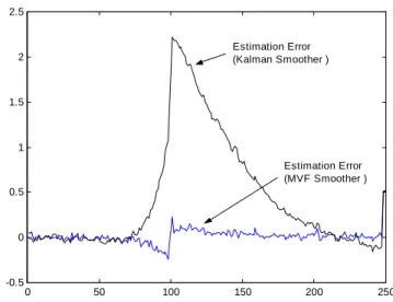
Figure (1) compares the robustness between the proposed MVF smoother and fixed-lag Kalman smoother which given temporary modeling uncertainty (35) for the second state which is related to turbine temperature. It is seen that the estimation error of the MVF smoother is remarkably smaller than that of the fixed-lag Kalman smoother on the inter-val where modeling uncertainty exists. In addition, it is shown that the estimation error is converged much faster than that of the fixed-lag Kalman smoother after temporary modeling uncertainty disappears. Therefore, the proposed MVF smoother is very useful than IIR type estimators when there exist temporary modelling errors and numerical errors. In Figure(2), the estimates of MVF smoother and filter are

0 50 100 150 200 250 -0.5 0 0.5 1 1.5 2 2.5 Estimation Error (MVF Smoother ) Estimation Error (Kalman Smoother ) 0 50 100 150 200 250 -0.5 0 0.5 1 1.5 2 2.5 Estimation Error (MVF Smoother ) Estimation Error (Kalman Smoother )

Fig. 1. Estimation errors of MVF smoother and Fixed-lag Kalman smoother 0 50 100 150 200 250 -0.5 0 0.5 1 1.5 2 2.5 3 3.5 dot : MVF Filter Solid : MVF Smoother Real State

Fig. 2. Estimates of MVF smoother and MVF filter ( h = 0 )

compared when the delay factor in MVF smoother is equal to zero. This means that the future data values are not used to estimate the state. Therefore, MVF filter is the special forms of MVF smoother when no future data values are used to estimate the state.

4. Conclusion

In this paper, the finite impulse response (FIR) smoother is proposed for discrete-time systems. The proposed smoother is chosen to optimize the minimum variance performance criterion with unbiased constraint. They are designed with linearity, unbiasedness, FIR structure, and independence of the initial state information.

The approaches of MVF smoother are logical and system-atic, while the existing result has heuristic assumption, such as infinite covariance of the initial state. Since there are few result and theoretical approaches on FIR smoother for model

(5)

based signal, this approaches have a great significance. Ad-ditionally, it is meaningful that the proposed MVF smoother is based on the general system that may have the singular system matrix and has both system and measurement noises. Thorough simulation studies, it is shown that the MVF fil-ter is the special forms of MVF smoother when no future data values are used to estimate the signal. It means that the proposed MVF smoother is generalized form of MVF fil-ter. The result of comparison between the proposed MVF smoother and fixed-lag Kalman smoother is also provided by simulation. It shows that the proposed MVF smoother is very useful for control problems than IIR type estimators when there are temporary modelling errors and numerical errors.

References

[1] V. R. Algazi, M. Suk, and C. S. Rim, ”Design of almost minimax FIR filters in one and two dimen- sions by WLS techniques”, IEEE Trans. Circuits Syst., vol. 33, pp. 590–596, 1986.

[2] M. O. Ahmad and J. D. Wang, ”An analytical least square solution to the design problem of two-dimensional FIR filters with quadrantally symmetric or antisymmetric frequency response”, IEEE Trans. Cir-cuits Syst., vol. 36, pp. 968–979, 1989.

[3] A.V. Oppenheim and R.W. Schafer, Digital signal

pro-cessing, Englewood Cliffs, NJ:Prentice-Hall, 1975.

[4] J. G. Proakis and D. G. Manolakis, Digital signal

pro-cessing principles, algorithms, and applications,

En-glewood Cliffs, NJ:Prentice-Hall, 1996.

[5] S. C. Pei and J. J. Shyu, ”Fast design of 2-D linear-phase complex FIR digital filters by analytical least squares methods” IEEE Trans. Signal Processing, vol. 44, pp. 3157–3161, 1996.

[6] S. Hosur and A. H. Tewfik, ”Wavelet transform domain adaptive FIR filtering”, IEEE Trans. Signal Processing, vol. 45, no. 3, pp. 617–630, 1997.

[7] Z. Wei-Ping, M. O. Ahmad, and M.N.S Swamy, ”Re-alization of 2-D linear phase FIR filters by using the singular value decomposition,” IEEE Trans. Signal Pro-cessing, vol. 47, no. 5, pp. 1349–1359, 1999.

[8] N. Damera-Venkata, B.L. Evans, and S.R. McCaslin, ”Design of optimal minimum-phase digital FIR filters using discrete Hilbert transforms”, IEEE Trans. Signal Processing, vol. 48, no. 6, pp. 1491–1495, 2000. [9] W. H. Kwon and O. K. Kwon, ”FIR filters and recursive

forms for continuous time-invariant state space mod-els”, IEEE Trans. Automat. Contr., vol. 32, pp. 352– 356, 1987.

[10] O. K. Kwon, W.H. Kwon, and K. S. Lee, ”FIR filters and recursive forms for discrete-time state space mod-els”, Automatica, vol. 25, pp.715–728, 1989.

[11] W. H. Kwon, K. S. Lee, and O. K. Kwon, ”Optimal FIR filters for time-varying state space models”, IEEE Trans. Aerosp. Electron. Syst., vol. 26, pp. 1011–1021, 1990.

[12] W. H. Kwon, K. S. Lee, and J. H. Lee, ”Fast algorithms

for optimal FIR filter and smoother for discrete-time state space models”, Automatica, vol. 30, pp. 489–492, 1994.

[13] R. W. Eustace, B.A.Woodyatt, G. L. Merrington, and A. Runacres, ”Fault signatures obtained from fault im-plant tests on an F404 engine”, ASME Trans. J. of En-gine, Gas Turbines, and Power, vol. 116, no. 1, pp.178– 183, 1994.