Assessment of genomic prediction accuracy using different selection and evaluation approaches in a simulated Korean beef cattle population

(1)

1912

This is an open-access article distributed under the terms of the Creative Commons Attribution License (http://creativecommons.org/licenses/by/4.0/), which permits unrestricted use, distribution, and

repro-duction in any medium, provided the original work is properly cited. www.ajas.info Asian-Australas J Anim Sci

Vol. 33, No. 12:1912-1921 December 2020 https://doi.org/10.5713/ajas.20.0217 pISSN 1011-2367 eISSN 1976-5517

Assessment of genomic prediction accuracy using different

selection and evaluation approaches in a simulated Korean beef

cattle population

Chiemela Peter Nwogwugwu1,a_{, Yeongkuk Kim}1,a_{, Hyunji Choi}1_{, Jun Heon Lee}1,_{*, and Seung-Hwan Lee}1,_*

Objective: This study assessed genomic prediction accuracies based on different selection methods, evaluation procedures, training population (TP) sizes, heritability (h2_{) levels, marker} densities and pedigree error (PE) rates in a simulated Korean beef cattle population.

Methods: A simulation was performed using two different selection methods, phenotypic and estimated breeding value (EBV), with an h2_{of 0.1, 0.3, or 0.5 and marker densities of} 10, 50, or 777K. A total of 275 males and 2,475 females were randomly selected from the last generation to simulate ten recent generations. The simulation of the PE dataset was modified using only the EBV method of selection with a marker density of 50K and a heritability of 0.3. The proportions of errors substituted were 10%, 20%, 30%, and 40%, res pectively. Genetic evaluations were performed using genomic best linear unbiased prediction (GBLUP) and single-step GBLUP (ssGBLUP) with different weighted values. The accuracies of the predictions were determined.

Results: Compared with phenotypic selection, the results revealed that the prediction accuracies obtained using GBLUP and ssGBLUP increased across heritability levels and TP sizes during EBV selection. However, an increase in the marker density did not yield higher accuracy in either method except when the h2_{was 0.3 under the EBV selection} method. Based on EBV selection with a heritability of 0.1 and a marker density of 10K, GBLUP and ssGBLUP_0.95 prediction accuracy was higher than that obtained by pheno-typic selection. The prediction accuracies from ssGBLUP_0.95 outperformed those from the GBLUP method across all scenarios. When errors were introduced into the pedigree dataset, the prediction accuracies were only minimally influenced across all scenarios.

Conclusion: Our study suggests that the use of ssGBLUP_0.95, EBV selection, and low marker density could help improve genetic gains in beef cattle.

Keywords: Heritability; Marker Density; Prediction Accuracy; Simulation; Selection Method

INTRODUCTION

Genomic estimated breeding values (GEBVs) of selected individuals are frequently used to improve the genetics of economically important traits in livestock species. These values incorporate the results of evaluations using genomic data, pedigree records and the phe-notypic performance of individuals using the best linear unbiased prediction (BLUP) or genomic method [1,2]. The accuracy of estimated breeding value (EBV) is an important factor that could influence the selection accuracy of breeding animals [3]. Alternatively, accuracy based on genomic selection (GS) could increase the predictive ability of the GEBV by applying single nucleotide polymorphism (SNP) information. Previous studies have reported improved GEBV accuracy, genetic gain, selection accuracy and a reduction in the generation interval for economic traits [2,4,5]. Calus [6] reported that the efficiency of GS

* Corresponding Authors: Jun Heon Lee

Tel: +82-42-821-5779, Fax: +82-42-825-9754, E-mail: [email protected]

Seung Hwan Lee

Tel: +82-42-821-5772, Fax: +82-42-821-5781, E-mail: [email protected]

1 _{Division of Animal and Dairy Science, Chungnam} National University, Daejeon 34134, Korea a_{These authors equally contribute to this study.} ORCID

Chiemela Peter Nwogwugwu https://orcid.org/0000-0001-7904-3991 Yeongkuk Kim

https://orcid.org/0000-0002-6530-2304 Hyunji Choi

https://orcid.org/0000-0001-9782-6586 Jun Heon Lee

https://orcid.org/0000-0003-3996-9209 Seung-Hwan Lee

https://orcid.org/0000-0003-1508-4887 Submitted Apr 9, 2019; Revised Jun 3, 2019; Accepted Jun 12, 2019

(2)

www.ajas.info 1913

Nwogwugwu et al(2020) Asian-Australas J Anim Sci 33:1912-1921

in livestock depends on the prediction accuracy of GEBVs. However, the prediction accuracy of GEBVs can be influenced by several factors, such as methods of prediction [7], the train-ing population (TP) size [6], the h2 of the trait [8] and the marker density [9]. An effect of errors in pedigree on the ac-curacy of the EBV has been reported in Korean Hanwoo cattle [10], but the use of genomic information could improve the accuracy of GEBVs.

Several authors have reported genomic prediction evalu-ation methods that could increase the accuracy of GEBVs. Hayes et al [2] and VanRaden [11] suggested the use of GBLUP, which employs genomic information in the form of a genomic relationship matrix. It also describes additive genetic cova-riance between individuals. GBLUP calculates direct genomic values (DGV) for genotyped individuals and has advantages over BLUP because marker density captures the Mendelian sampling across the genome. GBLUP is a straightforward procedure with low computational requirements, and has been used for genomic evaluations in cattle [12]. In contrast, single-step GBLUP (ssGBLUP) predicts how non-genotyped individuals can benefit from genomic information. The pedi-gree record and marker (SNPs) relationship matrices are combined in ssGBLUP, permitting the blending of geno-typed and non-genogeno-typed individuals in the genetic evaluation [13]. Weight (w) has been added to the genomic relationship matrix (G) [11], and such an adjustment may be interpreted as relative weight on the polygenic effect [14]. To facilitate inversion, w values between 0.90 and 1.0 indicate variations in prediction accuracy [11], but insignificant differences in EBVs have been reported when w ranges between 0.95 and 0.98 [14]. Recent studies have reported improved accuracies of GEBVs obtained using ssGBLUP compared with those from GBLUP in simulated beef cattle [15].

Korean Hanwoo cattle possess good meat flavour, tender-ness and taste, and efforts have been made to improve the quantity and quality of the carcass [16]. Applying GS is a po-tential approach to improve the genetic gains in economically important traits. However, Onogi et al [17] pointed out that the use of ssGBLUP for genomic evaluations is still emerging in beef cattle due to the greater complexity of their records compared with those of other livestock species, such as the existence of pedigree errors (PEs) and fewer full or half-sib families [10,18]. On the other hand, a simulation study allows the testing of several theories, permitting an unravelling of the complex evolutionary patterns that are otherwise difficult to comprehend. For example, the history of human migra-tion provides significant insight into the present patterns of DNA variation in humans [19]. Simulation studies in beef cattle and other livestock have provided information on their potential for genomic evaluation. They have also been used in studies of predictions of total genetic value [8], genomic prediction of simulated multi-breed and purebred cattle [20],

GS accuracy in simulated populations [21] and a comparison between single- and two-step GBLUP methods in simulated beef cattle [15]. These authors reported that GS increases the accuracy of the selection and economic benefits of the breed-ing objective durbreed-ing beef production. Therefore, the present study assessed the prediction accuracy of GEBV based on dif-ferent selection methods, evaluation procedures, TP sizes, h2 levels, marker densities and PE rates using a simulated Korean beef cattle population.

MATERIALS AND METHODS

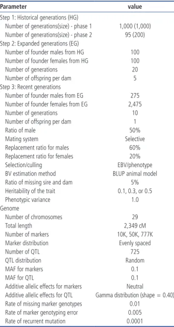
Simulation

Phenotypic and genotypic data were simulated using QMSim software [22] to mimic the actual structure and extent of linkage disequilibrium (LD) that exist in beef cattle [21]. Table 1 summarises the population structure and parameters of the simulation process. Marker densities of 10K, 50K, and 777K were simulated to generate bi-allelic markers distributed across 29 autosomal chromosomes of equal length. First, a his-torical population (HP) was simulated, which was comprised of constant size of 1,000 individuals across 1,000 generations. The size was gradually reduced to 200 individuals (100 males and 100 females) in the subsequent 95 generations to create initial LD and mutation-drift equilibrium. In addition, the HP was based on random mating. Next, 200 individuals (effective population size, Ne) were randomly selected from the last historical generation to expand the population size. All males and females were randomly mated and each dam produced five offspring per generation for 20 generations. Finally, 275 males and 2,475 females were randomly chosen from the expanded population. These selected individuals were simulated across ten recent generations with one off-spring per dam. Parameters that mimic Korean beef cattle were applied in the simulation based on the recent generations. Selection designs were based on the phenotypic performance and BLUP (EBV) approaches. The replacement ratios were 60% (sires) and 20% (dams). The rate of missing sire and dam records was 0.05. Traits with heritability levels of 0.1, 0.3, and 0.5 with a phenotypic variance of 1 were used. The Henderson mixed linear model was used to predict the EBVs, and the TP sizes were 1,000, 2,000, 3,000, and 5,000 indi-viduals randomly selected from generations 7, 8, and 9 [1]. A total of 200 individuals were randomly selected from the tenth generation for the prediction set. The scenarios con-sidered incorporated various selection methods, evaluation procedures, TP sizes, h2_{levels and marker densities.} Genome: The genome was comprised of 29 pairs of chro-mosomes with length identical to the actual bovine genome size (2,349 cM). Marker densities of 10K, 50K, and 777K were selected such that they would produce three different densities of segregating bi-allelic loci. The effect of the markers

(3)

1914 www.ajas.info

on the traits was neutral. The whole genome consisted of 725 quantitative trait loci (QTLs), and the segregating QTLs were comprised of two, three or four alleles randomly distributed with mean allelic frequency >0.01. The additive genetic effects of the QTLs were sampled from a gamma distribution with a parametric shape equal to 0.4. The rate of missing marker genotypes was 0.01, and the rate of marker genotyping error was 0.005. To establish mutation-drift equilibrium, a recurrent mutation rate of 10–5_{was used for the markers and the QTLs} throughout the simulation. The phenotypes were produced by adding random residuals to the QTL effects.

Simulation of pedigree errors

The simulation was performed based on the EBV selection

method with a 50K marker density and heritability of 0.3, as previously explained above. However, the protocol was modi-fied by introducing errors into the simulated pedigree dataset by randomly assigning sires to all progenies from generations 1 to 10, respectively. This method changed the sires’ infor-mation and resulted in wrong sire records. Thus, the impact of PEs was assessed in generations 7, 8, and 9 with their av-erages. The SampleBy function in the doBy package of the R software package (The R Foundation for Statistical Com-puting, Vienna, Austria) was used for creating PEs. Several error rates were substituted in the pedigree dataset for each generation, such as 10%, 20%, 30%, and 40%, respectively, as described previously by Oliehoek and Bijma [23] and adopted by Nwogwugwu et al [10].

Methods for genomic prediction

GBLUP procedure: The genotyped individuals were used to estimate the DGVs using the following model:

y = 1μ+Zg+e,

where y, µ, g, and e are the vectors of the phenotypes, overall mean, DGV and residual errors, respectively, and Z is the incidence matrix that relates phenotypes to random marker effects (DGVs). g ~

6

adding random residuals to the QTL effects.

136 137

138

The simulation was performed based on the EBV selection method with a 50K marker density and

139

heritability of 0.3, as previously explained above. However, the protocol was modified by introducing

140

errors into the simulated pedigree dataset by randomly assigning sires to all progenies from generations

141

1 to 10, respectively. This method changed the sires’ information and resulted in wrong sire records.

142

Thus, the impact of PEs was assessed in generations 7, 8, and 9 with their averages. The SampleBy

143

function in the doBy package of the R software package (The R Foundation for Statistical Computing,

144

Vienna, Austria) was used for creating PEs. Several error rates were substituted in the pedigree dataset

145

for each generation, such as 10%, 20%, 30%, and 40%, respectively, as described previously by

146

Oliehoek and Bijma [23] and adopted by Nwogwugwu et al [10]. 147

148

149

GBLUP procedure: The genotyped individuals were used to estimate the DGVs using the following

150 model: 151 152 y = 1μ+Zg+e 153 154

where y, µ, g, and e are the vectors of the phenotypes, overall mean, DGV and residual errors,

155

respectively, and Z is the incidence matrix that relates phenotypes to random marker effects (DGVs). g

156

~ N (0, 𝐺𝐺σ𝑔𝑔2), where σ𝑔𝑔2 is the additive genetic variance and g is the marker-based genomic 157

relationship matrix [11]. Random residuals were assumed such that e ~ N (0, Iσ𝑒𝑒2), where σ𝑒𝑒2 is the 158

residual variance. The G matrix was calculated using the SNP genotype data as follows:

159 160 G = (M − P)(M − P)′ 2 ∑𝑚𝑚𝑗𝑗=1𝑃𝑃𝑃𝑃(1 − Pj ) 161 , where 6

136 137

138

139

140

141

142

143

144

145

146

148

149

150 model: 151 152 y = 1μ+Zg+e 153 154

155

156

159 160 G = (M − P)(M − P)′ 2 ∑𝑚𝑚𝑗𝑗=1𝑃𝑃𝑃𝑃(1 − Pj ) 161 is the additive genetic variance and g is the marker-based genomic relation-ship matrix [11]. Random residuals were assumed such that e ~

6

136 137

138

139

140

141

142

143

144

145

146

148

149

150 model: 151 152 y = 1μ+Zg+e 153 154

155

156

159 160 G =_{2 ∑}(M − P)(M − P)_{𝑃𝑃𝑃𝑃(1 − P} ′ j ) 𝑚𝑚 𝑗𝑗=1 161 , where 6

136 137

138

139

140

141

142

143

144

145

146

148

149

150 model: 151 152 y = 1μ+Zg+e 153 154

155

156

159 160 G =_{2 ∑}(M − P)(M − P)_{𝑃𝑃𝑃𝑃(1 − P}′ j ) 𝑚𝑚 𝑗𝑗=1 161

is the residual variance. The G ma-trix was calculated using the SNP genotype data as follows:

6

adding random residuals to the QTL effects. 136

137

138

The simulation was performed based on the EBV selection method with a 50K marker density and 139

heritability of 0.3, as previously explained above. However, the protocol was modified by introducing 140

errors into the simulated pedigree dataset by randomly assigning sires to all progenies from generations 141

1 to 10, respectively. This method changed the sires’ information and resulted in wrong sire records. 142

Thus, the impact of PEs was assessed in generations 7, 8, and 9 with their averages. The SampleBy 143

function in the doBy package of the R software package (The R Foundation for Statistical Computing, 144

Vienna, Austria) was used for creating PEs. Several error rates were substituted in the pedigree dataset 145

for each generation, such as 10%, 20%, 30%, and 40%, respectively, as described previously by 146

Oliehoek and Bijma [23] and adopted by Nwogwugwu et al [10].

147 148

149

150 model: 151 152 y = 1μ+Zg+e 153 154

where y, µ, g, and e are the vectors of the phenotypes, overall mean, DGV and residual errors, 155

respectively, and Z is the incidence matrix that relates phenotypes to random marker effects (DGVs). g 156

residual variance. The G matrix was calculated using the SNP genotype data as follows: 159

160

G = (M − P)(M − P)′

2 ∑𝑚𝑚𝑗𝑗=1𝑃𝑃𝑃𝑃(1 − Pj ) 161

where M is the marker allele matrix for each individual and P is a matrix comprising the frequency of the second allele (pj), noted as 2(pj). GS3 software was used to perform the GBLUP analyses [24].

ssGBLUP procedure: This procedure employed data from genotyped and non-genotyped individuals and used the in-verse of the H matrix (H–1_{) to blend the pedigree-based matrix} (A) with the genomic relationship matrix (G) as described previously [25].

7

162

where M is the marker allele matrix for each individual and P is a matrix comprising the frequency of

163

the second allele (p𝙟𝙟), noted as 2(p𝙟𝙟). GS3 software was used to perform the GBLUP analyses [24].

164

ssGBLUP procedure: This procedure employed data from genotyped and non-genotyped

165

individuals and used the inverse of the H matrix (H–1_{) to blend the pedigree-based matrix (A) with the}

166

genomic relationship matrix (G) as described previously [25].

167 168 𝐻𝐻−1_{= 𝐴𝐴}−1_{+ (0} 0 0 (𝑤𝑤𝐺𝐺 + (1 − 𝑤𝑤)𝐴𝐴22)−1 − 𝐴𝐴22−1) 169 170

where w is a constant for the weighting factor as described by Abdalla et al [26], 𝐴𝐴22−1 is the inverse A

171

matrix for genotyped individuals and G is explained above. Three different weights (0.95, 0.90, and

172

0.85) were suggested to prevent possible problems with inversion and to explain the relative weight of

173

the polygenic effect required to describe the total additive variance. These different weight values are

174

indicated as ssGBLUP_0.95, ssSGBLUP_0.90, and ssGBLUP_0.85, respectively. For more

175

information, see [26]. The BLUPF90 software was used for the ssGBLUP predictions [27].

176 177

Accuracy of the prediction procedure

178

To evaluate the ability of genomic prediction for each set of marker densities, TP sizes of 1,000, 2,000,

179

3,000, and 5,000 individuals were randomly chosen from generations 7 to 9. In total, 200 individuals

180

were randomly selected from generation 10 for the prediction set. The accuracies of the predictions are

181

usually accessible from genetic evaluations and can be determined from the additive genetic variance

182

and the prediction error variance (PEV), as described previously [28]. The accuracy of GEBV was

183 calculated as: 184 185

√

1 − PEV

_σ

g 2 186

where w is a constant for the weighting factor as described by Abdalla et al [26],

7

162

163

164

165

166

167 168 𝐻𝐻−1_{= 𝐴𝐴}−1_{+ (0} 0 0 (𝑤𝑤𝐺𝐺 + (1 − 𝑤𝑤)𝐴𝐴22)−1 − 𝐴𝐴22−1) 169 170

where w is a constant for the weighting factor as described by Abdalla et al [26], 𝐴𝐴22−1 is the inverse A

171

172

173

174

175

176 177

178

179

180

181

182

183 calculated as: 184 185

√

1 − PEV

_σ

g 2 186

is the inverse A matrix for geno-typed individuals and G is explained above. Three different weights (0.95, 0.90, and 0.85) were suggested to prevent pos-sible problems with inversion and to explain the relative weight of the polygenic effect required to describe the total

Table 1. Population structure and simulation parameters

Parameter value

Step 1: Historical generations (HG)

Number of generations(size) - phase 1 1,000 (1,000) Number of generations(size) - phase 2 95 (200) Step 2: Expanded generations (EG)

Number of founder males from HG 100

Number of founder females from HG 100

Number of generations 20

Number of offspring per dam 5

Step 3: Recent generations

Number of founder males from EG 275

Number of founder females from EG 2,475

Number of generations 10

Number of offspring per dam 1

Ratio of male 50%

Mating system Selective

Replacement ratio for males 60%

Replacement ratio for females 20%

Selection/culling EBV/phenotype

BV estimation method BLUP animal model

Ratio of missing sire and dam 5%

Heritability of the trait 0.1, 0.3, or 0.5

Phenotypic variance 1.0

Genome

Number of chromosomes 29

Total length 2,349 cM

Number of markers 10K, 50K, 777K

Marker distribution Evenly spaced

Number of QTL 725

QTL distribution Random

MAF for markers 0.1

MAF for QTL 0.1

Additive allelic effects for markers Neutral

Additive allelic effects for QTL Gamma distribution (shape = 0.40)

Rate of missing marker genotypes 0.01

Rate of marker genotyping error 0.005

Rate of recurrent mutation 0.0001

(4)

additive variance. These different weight values are indicated as ssGBLUP_0.95, ssSGBLUP_0.90, and ssGBLUP_0.85, re-spectively. For more information, see [26]. The BLUPF90 software was used for the ssGBLUP predictions [27].

To evaluate the ability of genomic prediction for each set of marker densities, TP sizes of 1,000, 2,000, 3,000, and 5,000 individuals were randomly chosen from generations 7 to 9. In total, 200 individuals were randomly selected from genera-tion 10 for the predicgenera-tion set. The accuracies of the predicgenera-tions are usually accessible from genetic evaluations and can be determined from the additive genetic variance and the pre-diction error variance (PEV), as described previously [28]. The accuracy of GEBV was calculated as:

7

162

163

164

165

166

167 168 𝐻𝐻−1_{= 𝐴𝐴}−1_{+ (0} 0 0 (𝑤𝑤𝐺𝐺 + (1 − 𝑤𝑤)𝐴𝐴22)−1 − 𝐴𝐴22−1) 169 170

where w is a constant for the weighting factor as described by Abdalla et al [26], 𝐴𝐴22−1 is the inverse A 171

172

173

174

175

176 177

Accuracy of the prediction procedure 178

179

180

181

182

183 calculated as: 184 185 √1 − PEV_σ g 2 186

where PEV is the prediction error variance of EBV, and

8

187

where PEV is the prediction error variance of EBV, and σg2 is the additive genetic variance of each

188 trait. 189 190 RESULTS 191 192

Accuracy of genomic predictions based on phenotypic selection across all scenarios

193

Based on the phenotypic method of selection, the prediction accuracies for genomic evaluation were

194

estimated under different scenarios (e.g., 10K, 50K, and 777K; h2_{= 0.1, 0.3, and 0.5; different TP sizes),}

195

as shown in Table 2. The GBLUP prediction accuracies ranged from 0.312 to 0.563 for an h2_{of 0.1,}

196

0.475 to 0.735 for an h2_{of 0.3 and 0.575 to 0.808 for an h}2_{of 0.5, respectively. For ssGBLUP_0.95, the}

197

accuracies of prediction ranged from 0.341 to 0.566, 0.519 to 0.740, and 0.630 to 0.813 for heritabilities

198

of 0.1, 0.3, and 0.5, respectively. These results further indicate that the prediction accuracy of

199

ssGBLUP_0.95 increased by 8.77%, 4.30%, 2.06%, and 0.50% across TP sizes of 1,000, 2,000, 3,000,

200

and 5,000 with a heritability of 0.1 and a marker density of 10K when compared with GBLUP. The

201

prediction accuracy of GBLUP and ssGBLUP_0.95 dramatically increased with an increase in TP size.

202

The lowest accuracy was obtained for a TP size of 1,000, whereas the highest occurred with a TP size

203

of 5,000 individuals. An increase in the heritability level also improved the accuracy of prediction. The

204

lowest prediction accuracy was found for an h2_{of 0.1, whereas the highest was observed when the h}2

205

wasincreased to 0.5. In contrast, the prediction accuracy of the genomic methods did not improve with

206

an increase in the marker density. A 10K marker density showed better prediction accuracy, followed

207

by those of 50K and 777K. More precisely, the highest accuracy of genomic predictions was observed

208

when the marker density was 10K at an h2_{of 0.5 and a TP size of 5,000.}

209 210

Accuracy of genomic predictions based on EBV selection across all scenarios

211

Tables 3, 4, and 5 summarise the EBV method of selection and prediction accuracies for GBLUP and

212

ssGBLUP with three different combinations of weights (w) when the marker density ranged from 10K

213

is the additive genetic variance of each trait.

RESULTS

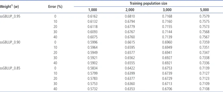
Accuracy of genomic predictions based on phenotypic selection across all scenarios

Based on the phenotypic method of selection, the prediction accuracies for genomic evaluation were estimated under dif-ferent scenarios (e.g., 10K, 50K, and 777K; h2_{= 0.1, 0.3, and} 0.5; different TP sizes), as shown in Table 2. The GBLUP pre-diction accuracies ranged from 0.312 to 0.563 for an h2_{of 0.1,}

0.475 to 0.735 for an h2_{of 0.3 and 0.575 to 0.808 for an h}2_of 0.5, respectively. For ssGBLUP_0.95, the accuracies of pre-diction ranged from 0.341 to 0.566, 0.519 to 0.740, and 0.630 to 0.813 for heritabilities of 0.1, 0.3, and 0.5, respectively. These results further indicate that the prediction accuracy of ssGBLUP _0.95 increased by 8.77%, 4.30%, 2.06%, and 0.50% across TP sizes of 1,000, 2,000, 3,000, and 5,000 with a heritability of 0.1 and a marker density of 10K when compared with GBLUP. The prediction accuracy of GBLUP and ssGBLUP_0.95 dra-matically increased with an increase in TP size. The lowest accuracy was obtained for a TP size of 1,000, whereas the highest occurred with a TP size of 5,000 individuals. An in-crease in the heritability level also improved the accuracy of prediction. The lowest prediction accuracy was found for an h2_{of 0.1, whereas the highest was observed when the h}2 was increased to 0.5. In contrast, the prediction accuracy of the genomic methods did not improve with an increase in the marker density. A 10K marker density showed better pre-diction accuracy, followed by those of 50K and 777K. More precisely, the highest accuracy of genomic predictions was observed when the marker density was 10K at an h2_{of 0.5} and a TP size of 5,000.

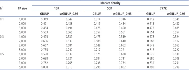
Accuracy of genomic predictions based on EBV selection across all scenarios

Tables 3, 4, and 5 summarise the EBV method of selection and prediction accuracies for GBLUP and ssGBLUP with three different combinations of weights (w) when the marker density ranged from 10K to 777K; h2_{= 0.1, 0.3, or 0.5; and} the TP size was varied between 1,000 and 5,000. The pre-diction accuracies for the GBLUP and ssGBLUP approaches using the EBV selection method were higher than those using

Table 2. Accuracies of genomic prediction using the GBLUP or ssGBLUP_0.95 procedures with the phenotypic selection method and various levels of heritability across TP sizes and marker densities

h2 _{TP size}

Marker density

10K 50K 777K

GBLUP ssGBLUP_0.95 GBLUP ssGBLUP_0.95 GBLUP ssGBLUP_0.95

0.1 1,000 0.319 0.347 0.314 0.346 0.312 0.341 2,000 0.421 0.438 0.415 0.434 0.413 0.430 3,000 0.484 0.494 0.478 0.490 0.473 0.485 5,000 0.563 0.566 0.557 0.561 0.551 0.554 0.3 1,000 0.495 0.539 0.475 0.519 0.478 0.524 2,000 0.606 0.630 0.588 0.610 0.588 0.612 3,000 0.667 0.681 0.648 0.662 0.649 0.662 5,000 0.735 0.740 0.717 0.721 0.717 0.722 0.5 1,000 0.590 0.639 0.575 0.630 0.575 0.630 2,000 0.698 0.721 0.684 0.711 0.680 0.708 3,000 0.752 0.765 0.738 0.754 0.734 0.751 5,000 0.808 0.813 0.796 0.802 0.793 0.799

GBLUP, genomic best linear unbiased prediction; ssGBLUP, single-step genomic best linear unbiased prediction with weight value of 0.95 (ssGBLUP_0.95: w = 0.95); TP, training population size.

(5)

Table 3. Accuracies of genomic prediction using the GBLUP or ssGBLUP procedures with three different combinations of weights (w) and the EBV selection method, various levels of heritability across TP sizes and a 10K marker density

h2 _{TP size} _GBLUP _{ssGBLUP_0.95}1) _{ssGBLUP_0.90}1) _{ssGBLUP_0.85}1)

0.1 1,000 0.369 0.404 0.389 0.374 2,000 0.470 0.490 0.472 0.454 3,000 0.531 0.542 0.522 0.503 5,000 0.605 0.606 0.586 0.565 0.3 1,000 0.526 0.570 0.552 0.533 2,000 0.633 0.656 0.635 0.614 3,000 0.690 0.703 0.681 0.659 5,000 0.753 0.757 0.734 0.712 0.5 1,000 0.622 0.664 0.644 0.624 2,000 0.722 0.742 0.720 0.698 3,000 0.770 0.782 0.759 0.737 5,000 0.822 0.827 0.804 0.782

GBLUP, genomic best linear unbiased prediction; ssGBLUP, single-step genomic best linear unbiased prediction; EBV, estimated breeding value; TP, training population size.

1)_{ssGBLUP_0.95, w = 0.95; ssGBLUP_0.90, w = 0.90; ssGBLUP_0.85, w = 0.85.}

Table 4. Accuracies of genomic prediction using the GBLUP or ssGBLUP procedures with three different combinations of weights (w) using the EBV selection method, various levels of heritability across TP sizes and a 50K marker density

0.1 1,000 0.360 0.401 0.387 0.372 2,000 0.465 0.485 0.467 0.449 3,000 0.523 0.535 0.516 0.497 5,000 0.596 0.597 0.577 0.557 0.3 1,000 0.532 0.577 0.559 0.540 2,000 0.638 0.660 0.640 0.619 3,000 0.693 0.706 0.684 0.662 5,000 0.754 0.758 0.736 0.714 0.5 1,000 0.611 0.658 0.638 0.619 2,000 0.710 0.733 0.712 0.690 3,000 0.760 0.773 0.751 0.729 5,000 0.812 0.817 0.795 0.773

1)_{ssGBLUP_0.95, w = 0.95; ssGBLUP_0.90, w = 0.90; ssGBLUP_0.85, w = 0.85.}

Table 5. Accuracies of genomic prediction using the GBLUP or ssGBLUP procedures with three different combinations of weights (w) using the EBV selection method, various levels of heritability across TP sizes and a 777K marker density

0.1 1,000 0.367 0.397 0.382 0.367 2,000 0.459 0.478 0.460 0.443 3,000 0.518 0.529 0.510 0.491 5,000 0.593 0.594 0.574 0.554 0.3 1,000 0.496 0.545 0.527 0.510 2,000 0.603 0.629 0.609 0.589 3,000 0.662 0.677 0.655 0.634 5,000 0.728 0.732 0.710 0.689 0.5 1,000 0.608 0.657 0.638 0.619 2,000 0.708 0.733 0.711 0.690 3,000 0.759 0.773 0.751 0.729 5,000 0.811 0.817 0.795 0.773

(6)

phenotypic selection. The prediction accuracies for GBLUP ranged from 0.367 to 0.605 for an h2_{of 0.1, 0.496 to 0.754} for an h2_{of 0.3 and 0.608 to 0.822 for an h}2_{of 0.5. ssGBLUP} 0.95 had an accuracy of 0.397 to 0.606 for an h2_{of 0.1, 0.545} to 0.758 for an h2_{of 0.3 and 0.657 to 0.827 for an h}2_{of 0.5.} The prediction accuracy was highest with ssGBLUP_0.95. These results indicate that the prediction accuracies obtained using ssGBLUP_0.95 increased by 9.48%, 4.25%, 2.07%, and 0.16% across TP sizes of 1,000, 2,000, 3,000 and 5,000 with a heritability of 0.1 and a marker density of 10K compared with those obtained using GBLUP. This study further re-vealed that the differences in prediction accuracy between ssGBLUP_0.95 and GBLUP were not large when the TP size was increased from 3,000 to 5,000. On the other hand, GBLUP increased by 15.67%, 11.63%, 9.71%, and 7.46% for TP sizes of 1,000, 2,000, 3,000, and 5,000 compared with phenotypic selection. The trend was similar for SSGLUP_0.95, but the increases were 16.2%, 11.87%, 9.71%, and 7.06%, respec-tively. The findings also show that increasing the number of genotyped animals in the TP sizes increased the prediction accuracies of GBLUP and ssGBLUP_0.95. Different levels of h2_{significantly influenced the prediction accuracy across} all scenarios. Increases in heritability also increased the pre-diction accuracy of the genomic evaluations. For example, changing the h2_{from 0.1 to 0.5 increased the accuracy of} GBLUP and ssGBLUP_0.95 by 84.95% and 84.14%, respec-tively, for a TP size of 1,000. The effect of marker density on the prediction accuracy of the GBLUP and ssGBLUP_0.95 methods followed a trend similar to that observed for phe-notypic selection. However, with an h2_{of 0.3 across all TP} sizes, the prediction accuracies for both evaluation methods

slightly increased from the 10K to 50K marker density but declined at 777K. The highest accuracy of genomic predic-tions was observed when the marker density was 10K, the h2_{was 0.5 and the TP size was 5,000.}

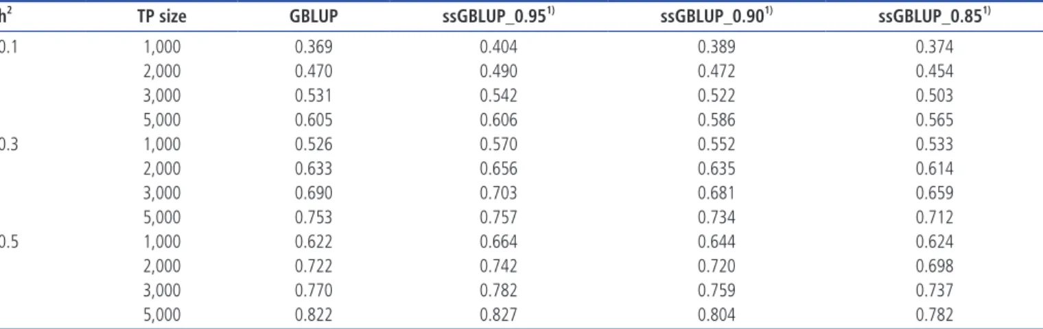
Accuracy of genomic predictions based on EBV selection under pedigree errors

The accuracy of predictions was investigated by introducing different proportions of error into a simulated pedigree da-taset while using a marker density of 50K, a heritability of 0.3, and three different weighted values of ssGBLUP (w = 0.95, 0.90, and 0.85) across the various TP sizes (Table 6). Intro-ducing errors into the pedigree dataset slightly affected the prediction accuracies across three different weights and TP sizes. The prediction accuracy was 0.6162 with no PE based on a TP size of 1,000 with ssGBLUP_0.95, but the accuracies slightly declined to 0.6132, 0.6118, 0.6093, and 0.6075 when errors were introduced at 10%, 20%, 30%, and 40%, respec-tively. With a 10% PE, the decline was 0.003. The results further revealed that the accuracy decreased to 0.0087 at 40% PE. The presence of PE somewhat affected the accuracy of prediction across TP sizes. However, as the TP size increased, the effect of PE on the prediction accuracy was insignificant.

DISCUSSION

In our study, we investigated the prediction accuracy of GEBV under different selection scenarios, evaluation procedures, TP sizes, heritability levels, marker densities and PE rates in a simulated Korean beef cattle population. Phenotypes are frequently used for selecting superior individuals in a

Table 6. Accuracies of genomic prediction based on EBV selection with various pedigree errors using a 50K marker density, an h2_{of 0.3, the ssGBLUP procedure and three}

different weight values

Weight1)_(w) _{Error (%)} Training population size

1,000 2,000 3,000 5,000 ssGBLUP_0.95 0 0.6162 0.6810 0.7168 0.7579 10 0.6132 0.6794 0.7160 0.7575 20 0.6118 0.6779 0.7155 0.7573 30 0.6093 0.6767 0.7144 0.7568 40 0.6075 0.6760 0.7139 0.7567 ssGBLUP_0.90 0 0.5996 0.6615 0.6960 0.7359 10 0.5964 0.6595 0.6949 0.7351 20 0.5949 0.6577 0.6941 0.7347 30 0.5921 0.6562 0.6927 0.7338 40 0.5902 0.6555 0.6921 0.7336 ssGBLUP_0.85 0 0.5834 0.6422 0.6753 0.7139 10 0.5799 0.6399 0.6739 0.7127 20 0.5783 0.6377 0.6729 0.7123 30 0.5753 0.6360 0.6713 0.7109 40 0.5732 0.6353 0.6706 0.7108

EBV, estimated breeding value; ssGBLUP, single-step genomic best linear unbiased prediction.

(7)

population. However, the statistical method of evaluation used is one factors that could influence the prediction ac-curacy of GEBV (Table 2). With phenotypic selection, there was a higher prediction accuracy for ssGBLUP_0.95 than for GBLUP, indicating that ssGBLUP_0.95 had advantages over GBLUP, possibly due to the combination of both geno-typed and non-genogeno-typed individuals. The combination could also help genomic markers capture any QTL effect or polygenic effect through EBVs [2,4]. Our results agree with those of Gowane et al [29], who obtained a higher predic-tion accuracy using ssGBLUP than GBLUP in a simulated population.

The accuracy of genomic prediction improved with greater numbers of individuals, as ssGBLUP showed a higher pre-diction accuracy than GBLUP at TP sizes of 1,000 to 3,000. However, when the TP size was 5,000, the results of both methods were comparable. The results further revealed that increasing the TP size across different scenarios improved the prediction accuracies. Several authors have reported improved accuracy for GEBVs when increasing the TP size in genotyped Holstein bulls [4] and simulated beef cattle [21].

The accuracy of the genomic predictions was affected by increased heritability. ssGBLUP showed a higher accuracy than GBLUP at all h2_{levels. Nwogwugwu et al [10] stated that} the higher the h2_{, the better the accuracy because h}2 repre-sents the strength of the association between the phenotype and breeding values. This implies that there is an association between h2_{and accuracy, as we observed; Kolbehdari et al} [30] reported similar results. Numerous studies have demon-strated increased accuracy with increasing h2_{values, which} agrees with our study [21,29].

The impact of marker density on the accuracy of genomic predictions has been examined in previous study [9]. With increases in marker density of 50K and 777K, the accuracies of the genomic evaluations did not improve. Zhu et al [31] reported limited prediction accuracy of a genomic evalua-tion with an increase in marker density from 0.5K to 20K in live weight, carcass weight and average daily gain. However, an increase in the marker density had a conflicting effect on prediction accuracy due to co-linearity between the effects of the markers in a simulated population [32]. Some authors have reported slightly improved accuracy of GEBVs with an increase in the marker density [21]. Nevertheless, these dif-ferences in results may be due to the genetic architecture or population structure.

The use of individual EBVs has greatly aided in animal genetic improvement. Therefore, selecting individuals based on the EBV could increase the accuracy of genomic predic-tions (Tables 3, 4, and 5). This study examined the prediction accuracies of GEBVs across multiple scenarios. The predic-tion accuracies of GBLUP and ssGBLUP_0.95 were higher when using EBV selection than when using phenotypic

se-lection. This could be attributed to the impact of the pedigree relationship among individuals, which facilitates accurate sire selection decisions. Our results agree with Amari [33], who previously stated that the EBV provides the most de-pendable information on the breeding results for a particular animal.

The performance of the ssGBLUP_0.95 method of predic-tion was superior to that of GBLUP in all scenarios. Therefore, combining genomic and pedigree data to predict traits im-proves accuracy, which leads to improved genetic gain in beef cattle breeding. However, GBLUP has been broadly utilised for genomic assessments in dairy cattle [7]. This assumes that the GBLUP method is mainly based on the LD between mark-ers and QTL. On the other hand, Meuwissen et al [8] proposed that an evaluation based on a combination of models improves the accuracy of prediction compared to methods that assume all SNPs have predictive value. Three different weights were added to ssGBLUP to solve the collinearity problem between variables and the low rank of the matrix, which could make inversion of the matrix difficult or impossible. ssGBLUP_0.95 had the highest prediction accuracy compared with weights 0.90 and 0.85. The prediction accuracy of ssGBLUP_0.90 was comparable with that of GBLUP in some scenarios. Less bias and a high prediction accuracy were reported by Vitezica et al [34] when the G matrix was adjusted with a weight factor using the ssGBLUP method. Similar observations have been reported in turkey [26]. The present findings further indi-cated significant differences in prediction accuracies among the weights used in this study and revealed that a weighting factor of 0.95 could be an optimal choice for genetic improve-ment. A higher accuracy of GEBV with ssGBLUP has been reported in Japanese black cattle [17], a simulated cattle pop-ulation [29] and Hanwoo beef cattle [35], indicating that the ssGBLUP method could be effectively used to improve traits with low heritability as well as traits that are difficult to mea-sure.

The present results indicate that the prediction accuracies of traits with a higher h2_{are more precise than those for traits} with a lower h2_{. This implies that the amount of additive} ge-netic variance explained by markers is small with a low h2_, thereby reducing the prediction accuracy [36]. The present study further investigated the effect of TP size on the pre-diction accuracy. The findings showed that the prepre-diction accuracy of genomic evaluations improved as the TP size increased, suggesting that the prediction accuracy tends to increase as information from an increasing number of in-dividuals is added. The results also indicate that the TP size is important for successful genomic prediction. Previous study has shown increased prediction accuracy with increasing TP size [4]. As shown in Tables 3, 4 and 5, that ssGBLUP_0.95 resulted in a higher accuracy at TP sizes of 1,000 to 2,000 individuals compared with GBLUP, and an even higher with

(8)

a TP size of 3,000; however, both methods were comparable above a TP size of 4,000. Our results fully agree with those of VanRaden et al [4], who observed that genomic gains increase almost linearly with an increase in TP size in Hol-stein bulls.

The effect of marker density on prediction accuracies was similar to that found for phenotypic selection. However, with an h2_{of 0.3, the prediction accuracies improved with an} in-crease in marker density of 50K, whereas the accuracy of prediction declined with the 777K marker. Genomic pre-dictions did not improve at 800K or in transcriptome panels over 50K in a pure-breed population [37]. Wang et al [38] also reported a similar result after increasing the marker den-sity from 0.05K to 3.2K, which greatly improved the genomic prediction accuracy, but there was less improvement when the marker density increased further. The present findings reveal high accuracies with a 10K marker density and a heri-tability of 0.1 and a TP size of 5,000; however, a heriheri-tability of 0.5 with a TP size of 5,000 produced the highest predic-tion accuracies in both models. The findings of the present study differ slightly from previous studies possibly due to variations in the genetic structure, marker density, TP size and method of evaluation.

Several authors have reported the effect of PEs on the EBV, the accuracy of the EBV and the genetic gain in livestock spe-cies [10,39]. Their findings indicate that PEs greatly reduce the accuracy of the EBV in beef and dairy cattle. However, introducing genomic information may resolve this reduction in the accuracy of the EBV or GEBV in livestock breeding. The results shown in Table 6 demonstrate the accuracy of predictions under PEs using a 50K marker density, an h2_of 0.3, and the use of ssGBLUP with three different weight val-ues (0.95, 0.90, and 0.85) across TP sizes. In this study, the prediction accuracy was only moderately influenced by dif-ferent weights and TP sizes. The findings further reveal that the prediction accuracy decreased consistently as more PEs were introduced into the data. This suggests that PEs have a negative relationship with prediction accuracy. Nwogwugwu et al [10] reported that the accuracy of the EBV decreased by 0.02 with a 40% PE from that generated with an estimate at 0% PE; however, with a 40% PE combined with genomic in-formation, the prediction accuracy of the GEBV declined by only 0.003 from that obtained using 0% PE and ssGBLUP_0.95. This indicates that the accuracy of prediction based on PE combined with genomic information is more reliable than the accuracy of EBV. With increasing TP size, the effect of PE on prediction accuracy was lower or negligible. This im-plies that additional information from relatives or increasing the TP size may improve the prediction accuracy, even if the pedigree is erroneous.

CONCLUSION

In general, selecting individuals based on the EBV had positive effects on the prediction accuracies of GEBVs compared with phenotypic selection, suggesting that assessing the pedigree records, phenotypic performance and genomic information of individuals improves the accuracy of GEBVs. Larger dif-ferences in the prediction accuracy between the GBLUP and ssGBLUP_0.95 methods were observed for traits with low heritability. This study showed that ssGBLUP_0.95 outper-formed GBLUP under all scenarios, and could be implemented for GS. Furthermore, increasing the TP size and h2_improved the prediction accuracies, whereas increasing the marker density did not improve accuracy of either method except in the case of a heritability of 0.3 and use of the EBV selec-tion method. This study further revealed that PE slightly influenced the prediction accuracies using different weights in ssGBLUP. The selection methods, evaluation procedures, TP sizes, h2_{levels, marker densities and PEs should be} con-sidered for genetic improvement and to properly implement GS in Korean Hanwoo breeding.

CONFLICT OF INTEREST

We certify that there is no conflict of interest with any financial organization regarding the material discussed in the manu-script.

ACKNOWLEDGMENTS

This study was carried out with the support of the AGENDA project for “Establishment and prediction model of marbling fineness index in Hanwoo (Project No. PJ012687022020)”. This study was carried out with the funding of Chungnam National University in Korea.

REFERENCES

1. Henderson CR. Best linear unbiased estimation and predic-tion under a selecpredic-tion model. Biometrics1975;31:423-47. 2. Hayes BJ, Bowman PJ, Chamberlain AJ, Goddard ME. Invited

review: Genomic selection in dairy cattle: progress and chall-enges. J Dairy Sci 2009;92:433-43. https://doi.org/10.3168/ jds.2008-1646

3. Van der Werf J. Principles of estimation of breeding values. In: Genetic evaluation and breeding program design. Armidale, Australia: University of New England; 2015. pp. 1-17. 4. VanRaden PM, Van Tassell CP, Wiggans GR, et al. Invited

review: Reliability of genomic predictions for North American Holstein bulls. J Dairy Sci 2009;92:16-24. https://doi.org/10. 3168/jds.2008-1514

(9)

paradigm shift in animal breeding. Anim Front 2016;6:6-14. https://doi.org/10.2527/af.2016-0002

6. Calus MPL. Genomic breeding value prediction: methods and procedures. Animal 2010;4:157-64. https://doi.org/10. 1017/S1751731109991352

7. Gao H, Christensen OF, Madsen P, et al. Comparison on genomic predictions using three GBLUP methods and two single-step blending methods in the Nordic Holstein popula-tion. Genet Sel Evol 2012;44:8. https://doi.org/10.1186/1297- 9686-44-8

8. Meuwissen THE, Hayes BJ, Goddard ME. Prediction of total genetic value using genome-wide dense marker maps. Genetics 2001;157:1819-29.

9. Solberg TR, Sonesson AK, Woolliams JA, Meuwissen THE. Genomic selection using different marker types and densities. J Anim Sci 2008;86:2447-54. https://doi.org/10.2527/jas.2007- 0010

10. Nwogwugwu CP, Kim Y, Chung YJ, et al. Effect of errors in pedigree on the accuracy of estimated breeding value for carcass traits in Korean Hanwoo cattle. Asian-Australas J Anim Sci 2020;33:1057-67. https://doi.org/10.5713/ajas.19.0021 11. VanRaden PM. Efficient methods to compute genomic

pre-dictions. J Dairy Sci 2008;91:4414-23. https://doi.org/10.3168/ jds.2007-0980

12. Habier D, Fernando RL, Dekkers JCM. The impact of genetic relationship information on genome-assisted breeding values. Genetics 2007;177:2389-97. https://doi.org/10.1534/genetics. 107.081190

13. Legarra A, Aguilar I, Misztal I. A relationship matrix including full pedigree and genomic information. J Dairy Sci 2009;92: 4656-63. https://doi.org/10.3168/jds.2009-2061

14. Christensen OF, Lund MS. Genomic prediction when some animals are not genotyped. Genet Sel Evol 2010;42:2. https:// doi.org/10.1186/1297-9686-42-2

15. Piccoli ML, Brito LF, Braccini J, et al. A comprehensive com-parison between single- and two-step GBLUP methods in a simulated beef cattle population. Can J Anim Sci 2018;98: 565-75. https://doi.org/10.1139/cjas-2017-0176

16. Song CW. The Korean Hanwoo beef cattle. Anim Genet Resour 1994;14:61-71. https://doi.org/10.1017/S1014233900000341 17. Onogi A, Ogino A, Komatsu T, et al. Genomic prediction in

Japanese Black cattle: application of a single-step approach to beef cattle. J Anim Sci 2014;92:1931-8. https://doi.org/10. 2527/jas.2014-7168

18. Legarra A, Christensen OF, Aguilar I, Misztal I. Single step, a general approach for genomic selection. Livest Sci 2014;166: 54-65. https://doi.org/10.1016/j.livsci.2014.04.029

19. Rogers AR, Wooding S, Huff CD, Batzer MA, Jorde LB. Ances-tral alleles and population origins: inferences depend on muta-tion rate. Mol Biol Evol 2007;24:990-7. https://doi.org/10. 1093/molbev/msm018

20. Kizilkaya K, Fernando RL, Garrick DJ. Genomic prediction

of simulated multibreed and purebred performance using observed fifty thousand single nucleotide polymorphism genotypes. J Anim Sci 2013;88:544-51. https://doi.org/10. 2527/jas.2009-2064

21. Brito FV, Neto JB, Sargolzaei M, Cobuci JA, Schenkel FS. Ac-curacy of genomic selection in simulated populations mimick-ing the extent of linkage disequilibrium in beef cattle. BMC Genet 2011;12:80. https://doi.org/10.1186/1471-2156-12-80 22. Sargolzaei M, Schenkel FS. QMSim: A large-scale genome

simulator for livestock. Bioinformatics 2009;25:680-1. https:// doi.org/10.1093/bioinformatics/btp045

23. Oliehoek PA, Bijma P. Effects of pedigree errors on the effi-ciency of conservation decisions. Genet Select Evol 2009;41:9. https://doi.org/10.1186/1297-9686-41-9

24. Legarra A, Ricard A, Filangi O. GS3: genomic selection, gibbs sampling, gauss seidel (and BayesCπ). Paris, France: INRA; 2014.

25. Christensen OF, Lund MS. Genomic prediction when some animals are not genotyped. Genet Sel Evol 2010;42:2. https:// doi.org/10.1186/1297-9686-42-2

26. Abdalla EEA, Schenkel FS, Emamgholi Begli H, et al. Single-step methodology for genomic evaluation in Turkeys (Meleagris gallopavo). Front Genet 2019;10:1248. https://doi.org/10.3389/ fgene.2019.01248

27. Misztal I, Tsuruta S, Lee DH, et al. BLUPF90 and related pro-grams (BGF90). In: Proceeding of the 7th World Congress on Genetics Applied to Livestock Production; 2002 Aug 19-23; Montpellier, France.

28. Misztal I, Wiggans GR. Approximation of prediction error variance in large-scale animal models. J Dairy Sci 1988;71: 27-32. https://doi.org/10.1016/S0022-0302(88)79976-2 29. Gowane GR, Lee SH, Clark S, Moghaddar N, Al-Mamun HA,

van der Werf JHJ. Effect of selection on bias and accuracy in genomic prediction of breeding values. bioRxiv 2018;298042. https://doi.org/10.1101/298042

30. Kolbehdari D, Schaeffer LR, Robinson JAB. Estimation of genome-wide haplotype effects in half-sib designs. J Anim Breed Genet 2007;124:356-61. https://doi.org/10.1111/j.1439- 0388.2007.00698.x

31. Zhu B, Zhang J, Niu H, et al. Effects of marker density and minor allele frequency on genomic prediction for growth traits in Chinese Simmental beef cattle. J Integr Agric 2017; 16:911-20. https://doi.org/10.1016/S2095-3119(16)61474-0 32. Muir WM. Comparison of genomic and traditional BLUP‐ estimated breeding value accuracy and selection response under alternative trait and genomic parameters. J Anim Breed Genet 2007;124:342-55. https://doi.org/10.1111/j.1439-0388. 2007.00700.x

33. Amari B. Understanding estimated breeding values [Internet]. Pinegowrie, Craighall, South Africa: Caxton House, 368 Jan Smuts Avenue; 2016 [2016 May 30]. Available from: https:// www.farmersweekly.co.za/farm-basics/how-to-livestock/

(10)

understanding-estimated-breeding-values/2016

34. Vitezica ZG, Aguilar I, Legarra A. One-step vs. multi-step methods for genomic prediction in presence of selection. In: Proceedings of the World Congress on Genetics Applied to Livestock Production. Volume genetic improvement pro-grammes: selection using molecular information - lecture sessions; 2010. No. 0131.

35. Lee J, Cheng H, Garrick D, et al. Comparison of alternative approaches to single-trait genomic prediction using geno-typed and non-genogeno-typed Hanwoo beef cattle. Genet Sel Evol 2017;49:2. https://doi.org/10.1186/s12711-016-0279-9 36. Goddard M, Hayes BJ. Genomic selection. J Anim Breed Genet

2007;124:323-30.

37. Erbe M, Hayes BJ, Matukumalli LK et al. Improving accuracy

of genomic predictions within and between dairy cattle breeds with imputed high-density single nucleotide polymorphism panels. J Dairy Sci 2012;95:4114-29. https://doi.org/10.3168/ jds.2011-5019

38. Wang Q, Yu Y, Yuan J, et al. Effects of marker density and popu lation structure on the genomic prediction accuracy for growth trait in Pacific white shrimp Litopenaeus vannamei. BMC Genet 2017;18:45. https://doi.org/10.1186/s12863-017- 0507-5

39. Israel C, Weller JI. Effect of misidentification on genetic gain and estimation of breeding value in dairy cattle populations. J Dairy Sci 2000;83:181-7. https://doi.org/10.3168/jds.S0022- 0302(00)74869-7