Least quantile squares method for the detection of outliers

Least quantile squares method for the detection of outliers

a_{Department of Applied Statistics, Konkuk University, Korea;} b_{Department of Applied Mathematics, Pukyong National University, Korea}

Abstract

k-least quantile of squares (k-LQS) estimates are a generalization of least median of squares (LMS) estimates.

They have not been used as much as LMS because their breakdown points become small as k increases. But if the size of outliers is assumed to be fixed LQS estimates yield a good fit to the majority of data and residuals calculated from LQS estimates can be a reliable tool to detect outliers. We propose to use LQS estimates for separating a clean set from the data in the context of outlyingness of the cases. Three procedures are suggested for the identification of outliers using LQS estimates. Examples are provided to illustrate the methods. A Monte Carlo study show that proposed methods are effective.

Keywords: influential case, least quantile squares, outliers, masking and swamping effects, re-gression diagnostics

1. Introduction

We consider a regression model with p independent variables (including the constant if there is an intercept)

Y = Xβ + ε,

where Y is an n× 1 vector of response, β is a p × 1 vector of unknown vector, X is an n × p matrix predictors, andε is an vector of random errors with zero mean and variance matrix is σ2_I

n. Linear

regression method has been commonly used to analyze data because of its simplicity and applicability. However, this methodology is susceptible to disturbing effect caused by some outliers contained in the data. Therefore, the detection and examination of outliers or influential cases are important parts of data analysis. In detecting multiple outliers, masking phenomenon or swamping phenomenon usually occurs and makes it difficult to find true outliers.

Many methods resistant to masking effect and swamping effect are suggested. Marasinghe (1985) suggested a multistage procedure to improve the computational complexity required to obtain the most likely outlier subset. A generalized extreme studentized residual (GESR) procedure was proposed by Paul and Fung (1991). Kianifard and Swallow (1989, 1990) proposed to use test statistics based on recursive residuals for identifying outliers. Atkinson (1994) suggested a fast method for the detection of multiple outliers by using forward search. Pena and Yohai (1999) proposed a method which is fast

This paper was supported by Konkuk University in 2020.

1_{Corresponding author: Department of Applied Mathematics, Pukyong National University, 45, Yongso-ro, Nam-Gu,}

Busan 48513, Korea. E-mail: myoon@pknu.ac.kr

Published 31 January 2021/ journal homepage: http://csam.or.kr c

and computationally feasible for a very large value of p. Jajo (2005) reviewed and compared outlier detection methods based on residuals.

One of general approaches for outlier detection is separating the data into a clean subset that is presumably free of outliers and a subset that contains all potential outliers. This approach is usually composed of several stages such as construction of a basic clean subset, calculation of residuals, outliers test and construction of a new clean subset. Hadi and Simonoff’s procedures (Hadi and Simonoff, 1993) adopted this approach and are summarized as follows.

A clean subset M of size s is constructed. The size of basic clean subset is s= int[(n + p − 1)/2]. Residuals di’s are calculated after fitting the model to the subset M. Residuals di’s correspond to the

internally studentized residuals for the cases included in M and the scaled prediction errors for others:

di=       yi− xT_iβˆM ˆ σM √ 1− xT i ( XT MXM )₋₁ xi , if i∈ M, yi− xTiβˆM ˆ σM √ 1+ xT i ( XT MXM )−1 xi , if i< M. (1.1)

Let|d|( j) be the jthorder statistic of the|di| in ascending order. If |d|(s+1) ≥ t(α/2(s+1),s−k), then the last (n− s) ordered cases are declared as outliers and the procedure stops. Otherwise, the procedure is re-peated with a new clean subset consisting of the first (s+1) ordered observations. If n = s+1 no outlier is declared. Two methods for constructing the basic clean subset were suggested. The first method initially fits a model to the full data by using least squares (LS) estimate, orders the observations by their standardized residuals and takes the first p ordered observations as the early basic subset. After fitting a model to the early basic subset a new basic subset is formed by taking the first (p+ 1) obser-vations ordered by the residuals corresponding to (1.1). The basic subset is increased systematically until the size of the subset equals to int[(n+ p − 1)/2]. The second method takes the backward-stepping approach (Rosner, 1975; Simonoff, 1988) based on the single linkage clustering (Hartigan 1981). A simulation study showed that the first method was more effective. Hadi and Simonoff (1993) demonstrated that their forward searching procedures are very effective and less affected by masking or swamping effects in comparison with other methods such as Marasinghe’s multistage procedure (1985), Paul and Fung’s (1991), and Kianifard and Swallow’s (1989, 1990) GESR procedure, OLS, and some high-breakdown methods like least median of squares (LMS) (Rousseeuw, 1984) and MM (Yohai, 1987).

The main purpose of this paper is to develop outliers detection methods which is invulnerable to masking and swamping effects. Newly suggested methods use least quantile squares (LQS) estimates for dividing the data into two groups, a clean set and an outlier set. LQS estimates are a generalization of LMS estimates. They have not been used as much as LMS because their breakdown points become small as the quartile value increases. But if the size of outliers is assumed to be fixed LQS estimates yield a good fit to the majority of data and residuals calculated from LQS estimates can be a reliable tool to detect outliers. In Section 2 the proposed methods are described with some examples. In Section 3 summary and concluding comments are presented.

2.

kkk

For detecting outliers it is important to estimate a model immune from the influence of the outliers. The widely used estimator of parameters in the regression model is the LS estimator which involves

the minimization of the sum of squared residuals. The drawback of the LS estimator is that it is sensitive to outliers in the data. A useful measure of the robustness of an estimator is the breakdown point of the estimator. Roughly speaking, it is the smallest fraction of arbitrary contamination that can cause the estimator to be infinite. For least squares, its breakdown points is 1/n which approaches zero as the sample size n increases.

Many robust estimators are suggested in the context of breakdown point. The most used high breakdown estimate is the LMS estimator, given by

arg min

θ med ri(θ),

where ri(θ) is the the residual of the ith observation. A generalization of the least median of squares

estimator is the LQS estimate, which minimizes the kthsmallest squared residual. We define k-LQS as arg min θ r 2 (k)(θ), where r2 (i)(θ) is the i th _{order statistic of r}2

(i)(θ)’s in descending order. Geometrically it corresponds to finding the narrowest strip covering k observations. The breakdown points of k-LQS decreases as k increases.

The computation of k-LQS estimates is complex. Several algorithms for LQS estimates have been proposed (Stromberg, 1993; Carrizosa and Plastria, 1995; Watson 1998). An LQS estimate involves determining Chebyshev solutions on all set of n+ 1 components. Stromberg (1993) used least squares and developed an algorithm to compute exact LQS estimates by considering ˆθ′s based on allnCp+1

possible subsets of size p+ 1. Watson (1998) provided alternative algorithms by using Gaussian elimination and modified linear programming.

We now propose new procedures for the identification of outliers in the regression by using k-LQS estimates. Residuals calculated from LQS estimates are used to separate the data into a clean subset and an outliers subset. The processes considered in this paper including Hadi and Simonoff’s perform the procedure for identifying outliers twice. One is for organizing a clean subset, and the other is for detecting candidates of outliers to be tested. Hadi and Simonoff used LS residuals in both procedures, but the two procedures need not be the same.

We suggest to use LQS residuals for constructing a clean set of M and then to use LS residuals di’s

in (1.1) for detecting and testing outliers. The test is performed using a t-distribution in this procedure. If LQS residuals are used in computing di’s in (1.1), the distribution of di’s under the null hypothesis is

not clear. Test procedure using LQS residuals needs p-values calculated by Monte Carlo simulations. The proposed procedures use k-LQS estimates using all observations in building a new clean subset, a new clean subset is formed independently from the previous clean subsets including the basic subset. However, Hadi and Simonoff’s procedure should organize a good basic subset because it uses the LS residuals calculated from the fitted model of the previous clean subset to build a new clean subset. The proposed methods are independent of the results of the previous stages and are expected to be more robust than Hadi and Simonoff’s procedure in building a clean set.

Three newly suggested procedures denoted as S1, S2, and S3 respectively are described as follows. Let “M1” denote Hadi and Simonoff’s procedure using the first method for building a basic clean subset.

S1: This method differ from M1 only in finding the basic clean subset. The basic clean subset is the set of observations with the smallest squared residuals calculated from k-LQS regression where k= int[(n + p − 1)/2].

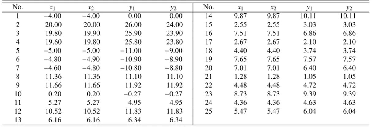
Table 1:Artificial data No. x1 x2 y1 y2 No. x1 x2 y1 y2 1 −4.00 −4.00 0.00 0.00 14 9.87 9.87 10.11 10.11 2 20.00 20.00 26.00 24.00 15 2.55 2.55 3.03 3.03 3 19.80 19.90 25.90 23.90 16 7.51 7.51 6.86 6.86 4 19.60 19.80 25.80 23.80 17 2.67 2.67 2.10 2.10 5 −5.00 −5.00 −11.00 −9.00 18 4.40 4.40 3.74 3.74 6 −4.80 −4.90 −10.90 −8.90 19 7.65 7.65 7.57 7.57 7 −4.60 −4.80 −10.80 −8.80 20 7.01 7.01 6.40 6.40 8 11.36 11.36 11.10 11.10 21 1.28 1.28 1.05 1.05 9 11.66 11.66 11.92 11.92 22 4.48 4.48 4.72 4.72 10 0.20 0.20 −0.27 −0.27 23 8.73 8.73 9.39 9.39 11 5.27 5.27 4.95 4.95 24 4.36 4.36 4.63 4.63 12 10.52 10.52 11.83 11.83 25 5.47 5.47 6.04 6.04 13 6.16 6.16 6.34 6.34

The second method uses LQS estimates for constructing both a basic clean subset and new clean subsets.

S2: The basic clean subset is obtained by the same method used in S1. After outlyingness test, if needed, a new clean subset of size k is constructed by using k-LQS estimates.

As a forward searching method neither LS, used in M1 nor LQS is perfect to avoid masking and swamping. The third method is designed to be relatively resistant to both masking and swamping effects which may occur in the process of S2. Let Ms denote the clean set of size s and Mcs be the

complement of Ms, the set of potential outliers of size (n−s). We calculate γs= n(Mcs∩Mcs₊₁)/n(M c s₊₁)

where n(Mi) is the size of Mi. Ifγsis small enough, it is highly probable that masking or swamping

occurred. Thus ifγsis small, both two subsets Msand Ms+1are used as clean sets. The Step 3 for S3

is described as follows.

S3: Find a basic clean subset by using LQS estimates, then compute and order residuals according to (1.1). If|d|(s+1) ≥ t(α/2(s+1),s−k), or|d|(s+1)< t(α/2(s+1),s−k)andγs ≥ δ for some fixed value of δ (we

useδ = 0.5), then form a new subset Ms+1by taking the (s+ 1) smallest residual observations

calculated from (s+1)-LQS regression. Otherwise, continue S2 procedure with a new subset Ms+1

and also perform M1 procedure with Msas a basic clean subset. The final outliers are determined

as the union of outliers detected by two procedures.

We now show an example to illustrate the proposed procedures. Columns x1and y1in the Table 1 have 25 observations. The regular observations are generated from the model Yi= Xi+εi, i= 8, . . . , 25

where Xi ∼ U(0, 15) and εi ∼ N(0, 0.52). Seven outliers, case 1–7 are perturbed at xi = −4,

xi = −5 + 0.2(i − 1) and Xi = 20 − 0.1(i − 1) to have Yi = Xi + 4 or Yi = Xi− 6 − 0.1(i − 1)

respectively. Outlyingness of 7 cases are obvious as we see in Figure 1. Columns x2 and y2 are obtained by modifying 7 outliers closer to the regular trend.

When columns x1and y1 are used S1, S2, and S3 correctly detected cases 1 to 7 as outliers but M1 identified only case 1 as an outlier. M1 fails because the basic clean subset contains none of true outliers. If columns x1and y2are used M1 and S1 detected only case 1 as an outlier, whereas S2 and S3 succeeded to detect 7 cases as outliers correctly. Table 2 and Table 3 contain subsets of outliers detected from the data of columns x2 and y2. The first column of the tables represents the size of subsets of outliers, decreasing from half of the data size down the table and the second column is the size of the clean subsets. The last column shows outcomes of the outlier test in which “Y” means

Figure 1:Scatter plot of X1and Y1in Table 1.

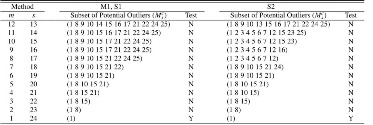
Table 2:Results of M1, S1 and S2 for the dataset of x1and y1in Table 1

Method M1, S1 S2

m s Subset of Potential Outliers (Mcs) Test Subset of Potential Outliers (Mcs) Test

12 13 (1 8 9 10 14 15 16 17 21 22 24 25) N (1 8 9 10 13 15 16 17 21 22 24 25) N 11 14 (1 8 9 10 15 16 17 21 22 24 25) N (1 2 3 4 5 6 7 12 15 23 25) N 10 15 (1 8 9 10 15 17 21 22 24 25) N (1 2 3 4 5 6 7 12 15 23) N 9 16 (1 8 9 10 15 17 21 22 24 25) N (1 2 3 4 5 6 7 12 16) N 8 17 (1 8 9 10 15 21 22 24 25) N (1 2 3 4 5 6 7 12) N 7 18 (1 8 9 10 15 21 22) N (1 8 9 10 15 21 24) N 6 19 (1 8 9 10 15 21) N (1 8 9 10 15 21) N 5 20 (1 8 10 15 21) N (1 8 10 15 21) N 4 21 (1 8 15 21) N (1 8 10 15) N 3 22 (1 8 15) N (1 8 15) N 2 23 (1 8) N (1 8) N 1 24 (1) Y (1) Y

Table 3:Results of M1 using Mc

14of S2 in Table 2 as a basic clean set

m s Subset of potential outliers (Mc

s) Test 11 14 (1 2 3 4 5 6 7 12 15 23 25) N 10 15 (1 2 3 4 5 6 7 12 15 23) N 9 16 (1 2 3 4 5 6 7 12 25) N 8 17 (1 2 3 4 5 6 7 12) N 7 18 (1 2 3 4 5 6 7) N

significant. M1 and S1 show the same results because they form the same basic clean subset of size 12. They failed to find the true outliers because the basic subset contains none of true outliers. S2 starts with a wrongly identified basic clean subset and chooses subsets of potential outliers successfully containing all of the true outliers in the early stages. But it eventually fails to detect the true outliers because swamping occurred at s = 18. By applying S3 to the data, S2 is executed and M1 is also executed with the basic clean subset M14 where M14 = {1 2 3 4 5 6 7 12 15 23 25} because Mc₁₄is quite different from M₁₃c = {1 8 9 10 13 15 16 17 21 22 24 25}. As seen in Table 3 M1 with a basic clean subset of M14detects{1 2 3 4 5 6 7} as outliers; consequently, the final detection of outliers

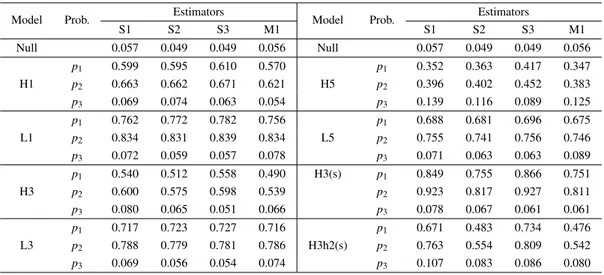
Table 4:Summary of Monte Carlo simulation

Model Prob. Estimators Model Prob. Estimators

S1 S2 S3 M1 S1 S2 S3 M1 Null 0.057 0.049 0.049 0.056 Null 0.057 0.049 0.049 0.056 p1 0.599 0.595 0.610 0.570 p1 0.352 0.363 0.417 0.347 H1 p2 0.663 0.662 0.671 0.621 H5 p2 0.396 0.402 0.452 0.383 p3 0.069 0.074 0.063 0.054 p3 0.139 0.116 0.089 0.125 p1 0.762 0.772 0.782 0.756 p1 0.688 0.681 0.696 0.675 L1 p2 0.834 0.831 0.839 0.834 L5 p2 0.755 0.741 0.756 0.746 p3 0.072 0.059 0.057 0.078 p3 0.071 0.063 0.063 0.089 p1 0.540 0.512 0.558 0.490 H3(s) p1 0.849 0.755 0.866 0.751 H3 p2 0.600 0.575 0.598 0.539 p2 0.923 0.817 0.927 0.811 p3 0.080 0.065 0.051 0.066 p3 0.078 0.067 0.061 0.061 p1 0.717 0.723 0.727 0.716 p1 0.671 0.483 0.734 0.476 L3 p2 0.788 0.779 0.781 0.786 H3h2(s) p2 0.763 0.554 0.809 0.542 p3 0.069 0.056 0.054 0.074 p3 0.107 0.083 0.086 0.080

using S3 is{1 2 3 4 5 6 7}, the union of {1 2 3 4 5 6 7} and {1}.

A Monte Carlo experiment for comparing the power of M1, S1, S2, and S3 are performed. We use the same outlier patterns and simulation scheme as used in Hadi and Simonoff (1993). The simulation results are limited because the pattern of the predictor, the position of outliers and the sample size are fixed. The data sets are generated from the model Yi = Xi+ εiwhere Xi ∼ U(0, 15)

andεi ∼ N(0, 12) except two models H3(s) and H3h2(s) which useεi ∼ N(0, 0.72). Outliers are

planted at Xi= 20 − 0.05(i − 1) for high leverage cases and at Xi= −7.5 + 0.05(i − 1) for low leverage

cases. The y values are given by Yi= Xi+ 4. Table 4 shows the simulation results.

The first column of Table 4 indicates models. H and L refer to high and low leverage outlier respectively, a number indicates the number of outliers and “s” indicates a model usingεi∼ N(0, 0.72).

Notations used in the second column are defined as: p1is the probability of identifying true outliers exactly. p2is the probability of identifying at least one true outlier. p3is the probability of identifying a clean observation as an outlier. The measures related to two negative effects of outliers are calculated as Pr(masking)= 1 − p2and Pr(swamping)= 1 − p3.

The first row of Table 4 shows that all methods control the size of Type I error at 0.05 approxi-mately. S1, S2, and S3 provided better overall performance than M1.

S3 gave the best results among the examined methods. S2 and S3 had a similar performance. The comparison of H3 and H3(s) shows that the difference in performance among M1, S1, S2 and S3 becomes larger if the ordinary observations are generated from the model with a small variance. The model H3h2(s) used a data set containing a group of 3 high leverage outliers and an additional group of 2 outliers positioned at lower right corner. The y values of two outliers are given by Yi= Xi− 4 for

xi= −5 + 0.05(i − 1) . The results of the model H3h2(s) show that the general patterns do not change

when there is more than one group of outliers.

Hadi and Simonoff’s procedure and the suggested methods have low breakdowns as n and p increase. But as the number of outliers is bigger and n is smaller, we can expect that the effect of LQS-residuals increases compared to LS-residuals in selecting a clean set. The proposed methods are applied to data sets having multiple predictors. We summarize the results.

predictors including four outliers. M1, S1, S2 and S3 succeed in identifying true outliers. Hawkins, Bradu and Kass data set (Hawkins et al., 1984) consists of 75 observations in three predictors. The first ten observations are high leverage outliers. Hadi and Simonoff reported that their method succeeded in detecting the cases 1–10 as outliers. But if the LMS approach is used in constructing a basic clean set, M1 identified cases 11, 12, 13, 14 as outliers. S1 also gave the same results whereas S2 and S3 correctly detected the outliers.

3. Summary and concluding remarks

In this article we have proposed three procedures for the identification of the outliers using k-LQS estimates. All three methods are related to the method proposed by Hadi and Simonoff (1993). The first method finds the basic clean subset using LQS estimates. The second method adopts the k-LQS approach for forming a clean subset of size k for the detection of outliers of size (n− k). The third method is designed to be more resistant to swamping or masking problems by combining the first method and the second method. The procedures search a fixed number of outliers using k-LQS esti-mates; however, they do not require presetting the size of outliers. The size of outliers are determined by t-tests for the no-outlier hypothesis.

As compared with other methods the LQS approach needs more computation. But in large re-gression problems a subsampling algorithm (Rousseeuw and Leroy, 1987) for approximating LQS estimates can be used to avoid excessive computation.

Acknowledgement

This paper was supported by Konkuk University in 2020.

References

Atkinson AC (1994). Fast very robust methods for the detection of multiple outliers, Journal of the American Statistical Association, 89, 1329–1339.

Carrizosa E and Plastria F (1995). The determination of a least quantile of squares regression line for all quantiles, Computational Statistics & Data Analysis, 20, 467–479.

Hadi AS and Simonoff JS (1993). Procedures for the identification of multiple outliers in linear models, Journal of the American Statistical Association, 88, 1264–1272.

Hartigan JA (1981). Consistency of single linkage for high-density clusters, Journal of the American Statistical Association, 76, 388–394.

Hawkins DM, Bradu D, and Kass GV (1984). Location of several outliers in multiple regression data using elemental sets, Technometrics, 26, 197–208.

Jajo Nethal K (2005). A review of robust regression and diagnostic procedures in linear regression, Acta Mathematicae Applicatae Sinica, 21, 209–224.

Kianifard F and Swallow WH (1989). Using recursive residuals, calculated on adaptive-ordered ob-servations, to identify outliers in linear regression, Biometrics, 45, 571–885.

Kianifard F and Swallow WH (1990). A Monte Carlo comparison of five procedures for identifying outliers in linear regression, Communications in Statistics - Theory and Methods, 19, 1913–1938. Marasinghe MG (1985). A multistage procedure for detecting several outliers in linear regression,

Technometrics, 27, 395–399.

Paul SR and Fung KY (1991). A generalized extreme studentized residual multiple-outlier-detection procedure in linear regression, Technometrics, 33, 339–348.

Pena D and Yohai VJ (1999). A fast procedure for outlier diagnostics in linear regression problems, Journal of the American Statistical Association, 94, 434–445.

Rosner B (1975). On the detection of many outliers, Technometrics, 17, 217–227.

Rousseeuw PJ (1984). Least median of squares regression, Journal of the American Statistical Asso-ciation, 79, 871–880.

Rousseeuw PJ and Leroy AM (1987). Robust Regression and Outlier Detection, John Wiley & Sons, New York.

Simonoff JS (1988). Detecting outlying cells in two-way contingency tables via backwards-stepping, Technometrics, 30, 339–345.

Stromberg AJ (1993). Computing the exact least median of squares estimate and stability diagnostics in multiple linear regression, SIAM Journal on Scientific Computing, 14, 1289–1299.

Watson GA (1998). On computing the least quantile of squares estimate, SIAM Journal on Scientific Computing, 19, 1125–1138.

Yohai VJ (1987). High breakdown-point and high efficiency robust estimates for regression, Annals of Statistics, 15, 642–656.