High-speed 3-D measurement with a large field
of view based on direct-view confocal microscope
with an electrically tunable lens
Hyeong-jun Jeong,1 Hongki Yoo,2 and DaeGab Gweon1,*
1Nano Opto-Mechatronics Laboratory, Department of Mechanical Engineering, Korea Advanced Institute of Science
and Technology (KAIST), 291 Daehak-ro, Yuseong-gu, Daejeon, 305-701, South Korea
2 Biomedical Optics and Photomedicine Laboratory, Department of Biomedical Engineering, Hanyang University,
222 Wangsimni-ro, Seongdong-gu, Seoul, 133-791, South Korea
2hyoo@hanyang.ac.kr
*gweondg@kaist.ac.kr
Abstract: We propose a new structure of confocal imaging system based
on a direct-view confocal microscope (DVCM) with an electrically tunable lens (ETL). Since it has no mechanical moving parts to scan both the lateral (x-y) and axial (z) directions, the DVCM with an ETL allows for high-speed 3-dimensional (3-D) imaging. Axial response and signal intensity of the DVCM were analyzed theoretically according to the pinhole characteristics. The system was designed to have an isotropic spatial resolution of 20 µm in both lateral and axial direction with a large field of view (FOV) of 10 × 10 mm. The FOV was maintained according to the various focal shifts as a result of an integrated design of an objective lens with the ETL. The developed system was calibrated to have linear focal shift over a range of 9 mm with an applied current to the ETL. The system performance of 3-D volume imaging was demonstrated using standard height specimens and a dental plaster.
©2016 Optical Society of America
OCIS codes: (120.3930) Metrological instrumentation; (120.6650) Surface measurements, figure; (110.6880) Three-dimensional image acquisition; (180.1790) Confocal microscopy. References and links
1. H. Leeghim, M. Ahn, and K. Kim, “Novel approach to optical profiler with gradient focal point methods,” Opt. Express 20(21), 23061–23073 (2012).
2. T. Kim, S. H. Kim, D. Do, H. Yoo, and D. Gweon, “Chromatic confocal microscopy with a novel wavelength detection method using transmittance,” Opt. Express 21(5), 6286–6294 (2013).
3. M. Ishihara and H. Sasaki, “High-speed surface measurement using a nonscanning multiple-beam confocal microscope,” Opt. Eng. 38(6), 1035 (1999).
4. H. Cui, N. Dai, W. Liao, and X. Cheng, “Intraoral 3D optical measurement system for tooth restoration,” Optik (Stuttg.) 124(12), 1142–1147 (2013).
5. M. F. M. Costa, “Surface inspection by an optical triangulation method,” Opt. Eng. 35(9), 2743 (1996). 6. M. S. Jeong and S. W. Kim, “Color grating projection moiré with time-integral fringe capturing for high-speed
3-D imaging,” Opt. Eng. 41(8), 1912 (2002).
7. M. C. Park and S. W. Kim, “Compensation of phase change on reflection in white-light interferometry for step height measurement,” Opt. Lett. 26(7), 420–422 (2001).
8. L. Deck and P. de Groot, “High-speed noncontact profiler based on scanning white-light interferometry,” Appl. Opt. 33(31), 7334–7338 (1994).
9. M. Gu, Principles of Three Dimensional Imaging in Confocal Microscopes (World Scientific, 1996). 10. G. Q. Xiao, T. R. Corle, and G. S. Kino, “Real-time confocal scanning optical microscope,” Appl. Phys. Lett.
53(8), 716–718 (1988).
11. A. Nakano, “Spinning-disk confocal microscopy -- a cutting-edge tool for imaging of membrane traffic,” Cell Struct. Funct. 27(5), 349–355 (2002).
12. K. Fujita, O. Nakamura, T. Kaneko, M. Oyamada, T. Takamatsu, and S. Kawata, “Confocal multipoint multiphoton excitation microscope with microlens and pinhole arrays,” Opt. Commun. 174(1-4), 7–12 (2000). 13. J. Bewersdorf, R. Pick, and S. W. Hell, “Multifocal multiphoton microscopy,” Opt. Lett. 23(9), 655–657 (1998). 14. T. Tanaami, S. Otsuki, N. Tomosada, Y. Kosugi, M. Shimizu, and H. Ishida, “High-speed 1-frame/ms scanning
15. M. D. Egger, R. Galambos, M. Hadravsky, and M. Petran, “Tandem-scanning reflected-light microscope,” JOSA A 58, 661–664 (1968).
16. H. J. Tiziani and H. M. Uhde, “Three-dimensional analysis by a microlens-array confocal arrangement,” Appl. Opt. 33(4), 567–572 (1994).
17. H. Buist, M. Müller, J. Squier, and G. J. Brakenhoff, “Real time two-photon absorption microscopy using multi point excitation,” J. Microsc. 192(2), 217–226 (1998).
18. G. J. Tearney, R. H. Webb, and B. E. Bouma, “Spectrally encoded confocal microscopy,” Opt. Lett. 23(15), 1152–1154 (1998).
19. C. Boudoux, S. Yun, W. Oh, W. White, N. Iftimia, M. Shishkov, B. Bouma, and G. Tearney, “Rapid wavelength-swept spectrally encoded confocal microscopy,” Opt. Express 13(20), 8214–8221 (2005). 20. J. Kim, D. Kang, and D. Gweon, “Spectrally encoded slit confocal microscopy,” Opt. Lett. 31(11), 1687–1689
(2006).
21. J. Liu, J. Tan, H. Bin, and Y. Wang, “Improved differential confocal microscopy with ultrahigh signal-to-noise ratio and reflectance disturbance resistibility,” Appl. Opt. 48(32), 6195–6201 (2009).
22. W. Zhao, J. Tan, and L. Qiu, “Bipolar absolute differential confocal approach to higher spatial resolution,” Opt. Express 12(21), 5013–5021 (2004).
23. D. R. Lee, Y. D. Kim, D. G. Gweon, and H. Yoo, “Dual-detection confocal fluorescence microscopy: fluorescence axial imaging without axial scanning,” Opt. Express 21(15), 17839–17848 (2013).
24. M. Browne, O. Akinyemi, and A. Boyde, “Confocal surface profiling utilizing chromatic aberration,” Scanning 14(3), 145–153 (1992).
25. G. Molesini, G. Pedrini, P. Poggi, and F. Quercioli, “Focus-wavelength encoded optical profilometer,” Opt. Commun. 49(4), 229–233 (1984).
26. M. D. Egger and M. Petrăn, “New reflected-light microscope for viewing unstained brain and ganglion cells,” Science 157(3786), 305–307 (1967).
27. J. M. Jabbour, B. H. Malik, C. Olsovsky, R. Cuenca, S. Cheng, J. A. Jo, Y. S. Cheng, J. M. Wright, and K. C. Maitland, “Optical axial scanning in confocal microscopy using an electrically tunable lens,” Biomed. Opt. Express 5(2), 645–652 (2014).
28. B. F. Grewe, F. F. Voigt, M. van ’t Hoff, and F. Helmchen, “Fast two-layer two-photon imaging of neuronal cell populations using an electrically tunable lens,” Biomed. Opt. Express 2(7), 2035–2046 (2011).
29. T. Wilson and S. J. Hewlett, “Optical sectioning strength of the direct-view microscope employing finite-sized pin-hole arrays,” J. Microsc. 163(2), 131–150 (1991).
30. T. Wilson and C. Sheppard, Theory and Practice of Scanning Optical Microscopy (Academic Press, 1984). 31. T. Wilson 1 and A. R. Carlini, “Size of the detector in confocal imaging systems,” Opt. Lett. 12(4), 227–229
(1987).
32. C. J. Sheppard and T. Wilson, “The theory of the direct-view confocal microscope,” J. Microsc. 124(2), 107–117 (1981).
33. Optotune, “Fast electrically tunable lens EL-10-30 series,” http://www.optotune.com/. 1. Introduction
The demand for accurately measuring the 3-dimensional (3-D) shape of various objects has been existing in many industrial and medical fields. Especially, the fast measurement technology of large-area and micro-surface is required in the inspection process of semiconductors, flat panel or plasma displays, and microelectromechanical systems [1–3]. In addition, large depth scanning range is needed in dental CAD/CAM industry [4]. As a result, to satisfy above requirements, various optical methods for high-speed 3-D surface measurement have been developed. The optical triangulation method has been used for a long time as a basis for 3-D sensing, but it is not suitable for micro-surface inspection [5]. Moiré interferometry also has a long history of development for 3-D contouring with a large field of view (FOV) and a high depth resolution with a few micrometers, however depth scanning range is restricted because of 2π ambiguity [6]. White light scanning interferometry produces a low coherence interferogram that permits precise measurement of object height without 2π ambiguity [7]. However, the measurement speed is not fast enough due to the need for mechanical axial scanning, and depth scanning range as well as spatial resolution are also limited by this actuator [8].
Confocal microscope is another popular method to measure 3-D surface by using optical sectioning capability. It has high spatial resolution due to a confocal pinhole which effectively eliminates out-of-focus noise [9]. Today, confocal microscope is widely used as a useful tool in various research and industrial fields. However, since the confocal method focuses on only one point in 3-D space, it is necessary to scan the beam or the object over lateral (x-y) and axial (z) directions for 3-D imaging. Thus it takes a lot of time to measure a 3-D shape of an object in conventional confocal scheme. To overcome this drawback, many novel structures
of confocal microscopy have been proposed to improve the scanning speed. Especially, multi-point illumination has been utilized to enhance the lateral scan speed by using micro-lens array and Nipkow disk [10–17]. Spectrally encoded confocal microscopy (SECM) is presented to replace one dimensional lateral scanning unit by encoding one dimensional spatial information of specimen in wavelength [18–20]. However, the SECM uses a quasi-monochromatic light source and disperse it by prisms or gratings that induce light loss. To improve the axial scanning speed in confocal microscope, differential confocal microscopy [21, 22], dual-detection confocal microscopy [23], and chromatic confocal microscopy (CCM) [24, 25] have been developed. However, depth measurement ranges are limited and the CCM suffers from low light efficiency in the same way as the SECM.
In this paper, we propose a new structure of confocal imaging system without mechanical scanning mechanism. It is based on a direct-view confocal microscope (DVCM) for the fast lateral (x-y) scanning with an electrically tunable lens (ETL) for the fast axial (z) scanning. DVCM was first invented by Egger et al. primarily for the examination of thick biological tissue [15, 26]. It employs a pinhole array to make many pairs of confocal points in the source and the detector plane respectively. We used an incoherent light source and a pinhole array instead of a laser and a microlens-pinhole array, to make a system simple, miniaturized, and inexpensive. An electrically tunable lens of which the focal length is varied with the applied electrical current is now commercially available. The uses of the ETL in confocal microscopes were already reported and verified its utility [27, 28]. In this study, to the best of our knowledge, we employed the ETL in the DVCM for the first time. This novel imaging method removes all the mechanical scanners from confocal microscopy, thus it has a capability of fast 3-D imaging. Also, the telecentric configuration of the objective lens with tunable focus achieves a constant field of view over a large 3-d volume.
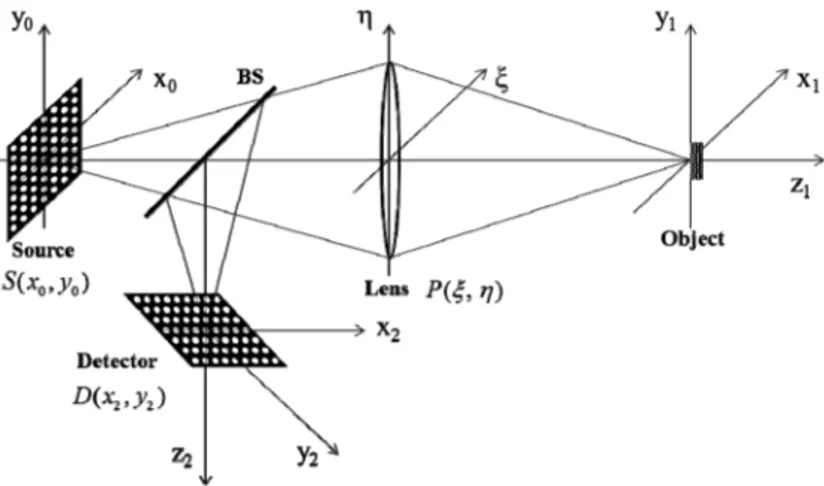
Fig. 1. Schematic of DVCM. A pinhole array is placed in the source plane (x0-y0) and the
generated source array is illuminated to the object plane (x1-y1). The reflected light from the
object is split by a beam splitter (BS) and observed in the detector plane(x2-y2). A lens has both
roles of objective lens and collector lens. It is assumed that the lens has a normalized pupil function P( , )ξ η having radius of one.
2. Principles
2.1 Direct-view confocal microscope (fast x-y scan method)
We first consider the structure of a DVCM theoretically and simulate its axial response according to the pinhole characteristics. Figure 1 shows the schematic of the DVCM. It employs many pairs of confocal points using a pinhole array in the source and detector planes so that it permits real-time visual imaging. These confocal pairs are arranged to be sufficiently far apart to ensure that light originating from one particular source point is
collected only by the corresponding detector point. It allows the optical sectioning property similar to that of the point scanning confocal microscope. As a result, the object is probed simultaneously in synchronism, one essentially have many confocal microscopes operating in parallel [29].
A pinhole array is illuminated by light from an incoherent source, then a multi-source array is generated in the source plane. This multi-source array is imaged to the object by a lens. The back-reflected light from the object is split by a beam splitter (BS) and forms an image in the detector plane. The detector plane is also composed of a pinhole array which coincides with the source array. The distribution of the pinhole arrays at the source and the detector planes respectively can be expressed as convolution of an on-axis pinhole function, and a two-dimensional comb function:
0 0 0 0 0 0 ( , ) ( , ) t w S t w H t w comb comb T T = ⊗ (1) and 2 2 2 2 2 2 ( , ) ( , ) t w , D t w H t w comb comb T T = ⊗ (2)
where ⊗is the 2-D convolution operation, and t and w are normalized optical coordinates
related to real lateral coordinates x and y via the expression t = (2π/λ)x sinα and w = (2π/λ)y sinα, respectively. Here λ denotes the free-space source wavelength and sin α denotes is the numerical aperture (NA) of the lens. T in the Eq. (1) and (2) means a pinhole separation and it is assumed that pinhole separations are the same along the t and w directions. H t w( , )denotes the on-axis pinhole function given by
2 2 2 1 ( , ) , 0 p t w v H t w otherwise + ≤ = (3)
where vp is the pinhole radius in normalized optical unit.
The light intensity distribution on the object plane then can be described as:
2 1( , , ) ( , ) 3 ( , , ) ,
I t w u =S t w ⊗ h t w u (4)
where ⊗3 denotes the three-dimensional convolution operation and h is the defocused
amplitude point-spread function of the lens and is given by [9, 30, 31]
( )
[ ]
( , , ) ( ', ', ) exp ' ' ' ',
h t w u =
Pξ η u i ξ t+η w dξ ηd (5)where P( ', ', )ξ η u represents the defocused pupil function in the normalized coordinate (ξ η', ') lies in the plane of the lens and can be written as:
(
2 2)
2 2 exp ' ' ' ' 1 ( ', ', ) 2 0 otherwise , iu Pξ η u = − ξ +η ξ +η ≤ (6)where u is a normalized axial optical coordinate representing defocus and is related to real axial distance, z, via the expression u = (8π/λ)z sin2(α/2). For the convenience to quantify the
axial response, we assume that a perfect planar mirror is placed at the object plane. Then the reflected light intensity formed in the detector plane can be described as [32]:
(
2)
(
2)(
2)
2( ) 1( , , ) 3 ( , , ) ( , ) 3 3 .
As shown in Eq. (7), the axial response to a perfect planar mirror in a DVCM is a function of the source and detector’s distribution and varying with the axial optical coordinate, u. Thus, the optical sectioning strength of DVCM depends on the characteristics of the pinhole array, i.e. pinhole size and pinhole separation. The source and detector are defined as Eq. (1) and Eq. (2), and the simulation results of axial responses according to the pinhole radius and the pinhole pitch are shown in Fig. 2.
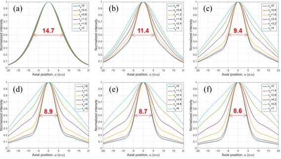
Fig. 2. Simulation results of axial responses according to pinhole radius (vp) and pinhole pitch (T). Each graph shows the axial responses according to the ratio of pinhole radius to pinhole pitch from 0.1 to 0.5, by 0.1 steps, when (a) T = 4, (b) T = 6, (c) T = 8, (d) T = 10, (e) T = 12 and (f) T = 14
The axial response curve become narrower when pinhole radius decreases at each case, as is well-known generally. In addition, the optical sectioning strength is improved as the pinhole pitch is increased, as the minimum full-width at half-maximum (FWHM) of the axial response decreases when the pinhole pitch increased (Fig. 2). This improvement is induced by the reduced cross-talks between pinholes when pinholes are more separated.
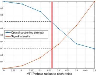
In addition to the optical sectioning strength, the signal intensity should be considered because the amount of light is reduced by a factor equal to the ratio of the area of the pinholes to its total area in the pinhole array. The straightforward ways to improve the signal level is to use large pinholes or to decrease the pinhole separation. These methods, however, cause to decrease the optical sectioning strength as discussed above. Therefore, one should find a proper design point in a trade-off between the optical sectioning strength and the signal intensity. We first determined the pinhole separation based on the analysis of the minimum FWHM (i.e. when the pinhole radius is zero) along the pinhole pitch. The minimum FWHM of the axial response is rapidly decreased until 10 optical unit of pinhole pitch and the variance is small after that point as shown in Fig. 2. Thus we analyzed the optical sectioning strength and the signal intensity when T is 10.
Fig. 3. Optical sectioning strength and signal intensity according to the ratio of pinhole radius to pinhole pitch when pinhole pitch (T) is fixed as 10. Optical sectioning strength is inversely proportional to the FWHM and normalized when r/T is 0. Signal intensity is proportional to the pinhole area and normalized when r/T is 0.5.
Figure 3 shows the optical sectioning strength and the signal intensity according to the ratio of pinhole radius to pinhole pitch. The optical sectioning strength is defined as the reciprocal of the FWHM of an axial response curve and the signal intensity is the ratio of a pinhole area (where the light can pass) to a unit area that is expressed as πvp2/T2. In this study,
we tried to get a high optical sectioning strength as possible with an allowable signal intensity. 30% of the signal intensity was enough to get images based on the analysis of the power of the source and the sensitivity of the photo sensor used in this work. Thus the 70% of the optical sectioning strength and the 30% of the signal intensity point was determined as the design value as marked in Fig. 3. The ratio of the pinhole radius to the pinhole pitch (vp/T) at
this point is 0.27.
2.2 Electrically tunable lens (fast z scan method)
Electrically tunable lens (ETL) can be used in fast z-scanning without mechanical moving parts where the focal length of the lens changes with an applied current. The ETL consists of a container filled with an optical fluid and sealed off with a flexible spherical membrane. An electromagnetic actuator is integrated in the lens, which controls a ring that exerts pressure on the container and squeezes more liquid into the lens volume. This leads to a bulging of the membrane. Therefore, the focal length of the lens can be controlled by the current flowing through the coil of the actuator [28]. ETLs with a varying focal length of a few tens of millimeters are commercially available with a few milliseconds response time and within 15 ms settling time. Also, the ETL is highly reproducible and stable, since the current through the coil directly induces a force, and there is no friction and no hysteresis [33]. Using an ETL with a negative offset lens (NOL) can make a focal tuning range from negative (diverging) to positive (converging) so that it is compatible with infinity-corrected optics.
The straightforward way to implement the ETL/NOL assembly is to mount it to the rear stop of the objective lens. It is simple and easy to implement and also available in commercial microscopes. If one try to place an ETL/NOL assembly to the rear stop of the commercial objective, however, it might be a suboptimal location because most objectives have an inaccessible aperture stop. It leads to non-telecentric condition that changes field-of-view (FOV) size or magnification if the axial focus position changes. Also the numerical aperture (NA) of the object space changes and thus the resolution is different over the focusing range. Thus we designed the objective lens, so that it is possible to position an ETL/NOL assembly
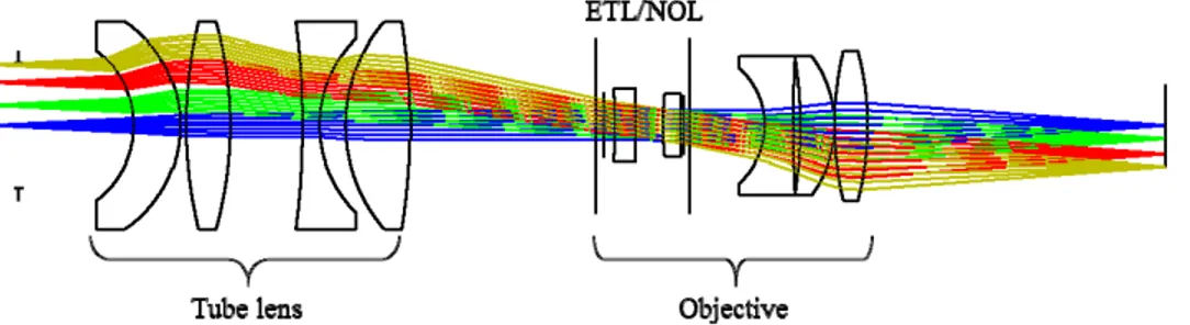
to an optimal place, i.e. the rear stop of the objective lens and those problems above will not arouse. The configuration is shown in Fig. 4.
Fig. 4. Implementation of an ETL/NOL with an objective lens and its focal shift in accordance with changing the radius of the ETL.
3. System design
3.1 Schematic of the experimental setup
A schematic diagram of the experimental setup of the direct-view confocal microscope (DVCM) with the ETL is shown in Fig. 5. The LED (M625L3, Thorlabs, NJ) was used as an incoherent light source and illuminated a pinhole array via an aspheric condenser lens (ACL2520-DG6-A, Thorlabs, NJ). The beam was p-polarized by a linear polarizer (LP, LPVIS100-MP2, Thorlabs, NJ). The pinhole array was manufactured by a printing method on a thin PET panel, i.e. making a film mask. The size of the pinhole array was 15 mm × 15 mm with 500 × 500 transparent circled array pattern. The separation of the pinhole to pinhole was 30 µm and the pinhole radius was determined as 8 µm according to the criteria established at section 2.1. Multi-source array illuminated the object through the relay optics.
The relay optics consists of a tube lens, an ETL/NOL assembly (EL-10-30-C, Optotune, Switzerland), an objective, and a quarter-wave plate (QWP, WPQ10E-633, Thorlabs, NJ). The relay optics was designed as double telecentric system so that the ETL/NOL assembly can be implemented to the rear aperture of the objective lens. The QWP plays a role of rotating the polarization amount of 90° between illumination and reflection light so that only reflection light goes to the detection optics by a polarizing beam splitter (PBS, CM1-PBS252, Thorlabs, NJ). In order to minimize unwanted light signal, such as reflected light from the surfaces of optical components, QWP was placed at the distal part of the optics. The reflected light from the object formed an image at the pinhole array and it was imaged again to the image sensor (acA2040-180km, Basler, Germany) through an imaging lens (Xenoplan 1.4/17, Schneider, Germany).
Fig. 5. Schematic of the experimental setup. CL: condenser lens, LP: linear polarizer, PBS: polarizing beam splitter, ETL: electrically tunable lens, QWP: quarter-wave plate.
3.2 Lens design
The goal of the optical system in this work was to develop a miniaturized instrument to measure a large volume of a 3-D object. The target field of view (FOV) was 10 mm × 10 mm with the depth scanning range of 5 mm. Because the size of the pinhole array was 15 mm × 15 mm, the magnification of the optical system determined by a tube lens and an objective should be 1.5. Also, the focal shift should be more than 5 mm according to the variance of the ETL’s curvature. The tube lens and the objective lens except the ETL were designed using an optical design software (ZEMAX, Radiant Zemax, WA) to minimize the aberration under the diffraction limit.
The final optics design is shown in Fig. 6. The total length of the optical system was 195 mm. The tube lens was composed of 4 spherical lenses and its effective focal length was 50.1 mm. The objective was composed of an ETL/NOL set and 3 spherical lenses, and its effective focal length and numerical aperture (NA) was 33.4 mm and 0.1, respectively. Thus the magnification of the optical system was 50.1 mm/33.4 mm = 1.5 as desired, which provided the FOV of 10 mm × 10 mm. The depth scanning range was 0 to 5.1 mm when the curvature of the ETL varied from 0.016 mm−1 to 0.030 mm−1. While the focal plane was shifting from
beginning to end, the change of the FOV was only 3 µm.
Fig. 6. Layout of the designed lens system. 4. Experiments
4.1 System calibration and axial response
We first performed a calibration to find a relation between the applied current into the ETL and the focal shift of the system. The curvature of the ETL varied by the driving current to the electrically tunable lens with a range of 0 to 400 mA, then the back focal length of the objective lens was changed accordingly. In order to find the focal shift, we attached a planar mirror to a motorized linear stage (MTS25/M-Z8, Thorlabs) and located the mirror to a specific position. Then we applied a triangular current signal to the ETL, so that the reflected signal from the mirror varied according to the current. When the reflected signal was maximum, the distance from the last surface of the objective lens to the mirror was regarded as the back focal length and the applied current signal at that time was recorded.
The calibration result is shown in Fig. 7(a). We set a z-position to zero at the first position of the planar mirror and moved it by 0.5 mm steps. Then we measured the current when the reflected intensity signal was maximum at each step. The z-position was linearly increased from 0 to 9 mm when the driving current was 0 to 350 mA. The linear model was expressed as Z = aI + b, where Z is the z-position with the applied current, I, and a and b are coefficients of the linear model. The values of the coefficients were a = 0.0279 and b =
−0.7021 with R2 = 0.9995 showing a good linear relation between the applied current and the
following z-position. Also, the absolute accuracy of the calibration of the axial scanning, defined as root mean square error (RMSE), was estimated to be 64 µm.
After the calibration, we evaluated an axial response of the planar mirror. The applied currents were converted to the axial positions from the calibration data and the normalized
intensities were plotted as shown in Fig. 7(b). The FWHM of the axial response was measured as 130 µm, which matched well to the theoretical value of 128 µm analyzed in chapter 2 (see Fig. 2).
Fig. 7. (a) Calibration result and (b) axial response of the system. 4.2 Step height measurements
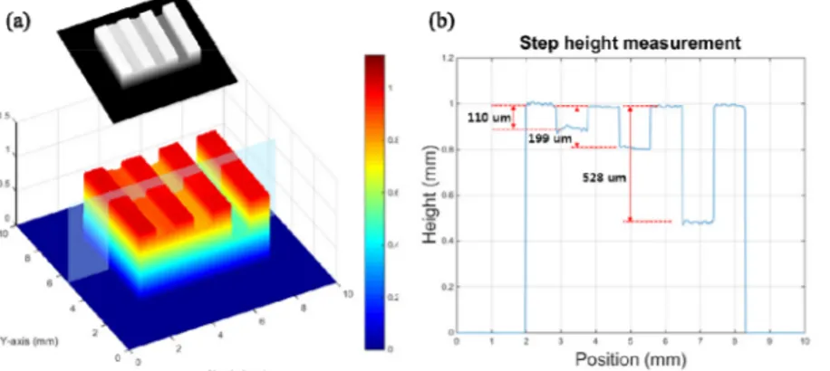
We measured a step height specimen and acquired its 3-D reconstruction image to evaluate a height measurement capability of the developed system. The specimen was designed and manufactured to have 100, 200 and 500 µm depth of grooves and each linewidth and space was 1 mm. It was certified by using a probe contact measuring system from Korea Polytechnic University. The certificated heights were 112.5, 213.9 and 516.3 µm, about 10 µm higher than designed values. To measure the height standard specimen, we acquired 200 2-D images using the DVCM with a step size of 5 µm covering a depth range of 1 mm. The measurement results are shown in Fig. 8. The rendered 3-D surface profile is shown in Fig. 8(a) and we can clearly observe the pattern with depth information. In order to analyze the depth measurement precision of the developed system, we measured the cross-sectional profiles of the specimen as shown in Fig. 8(b). The measured values were 110.0, 199.4 and 528.3 µm, resulting in error between the measured heights and certificated heights less than 20 µm.
Fig. 8. Measurement result of a step height specimen. (a) 3-D reconstructed image and (b) its cross-section profile.
In confocal reflectance microscopy, the axial resolution is affected by many factors, including width of axial response, signal-to-noise ratio, axial step size, and peak detection
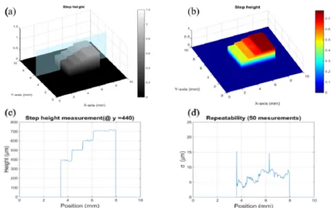
algorithm. One representative way to evaluate a precision of axial measurement is repeatability test by measuring specific points many times and calculating a standard deviation. The measurements were performed on a stair-step specimen with a step height of 100 µm. 200 2-D images were acquired with a step size of 5 µm within 2 sec. 3-D reconstructed images of the stair-step specimen are shown in Figs. 9(a) and 9(b) with gray scale and color-coded scale, respectively. In order to estimate a precision of height measurement, a cross-section of a certain position and its repeated measurements were analyzed. Figure 9(c) shows that the cross-sectional profile is well coincide with 100 µm steps. To demonstrate the repeatability, we repeated the measurement of this section 50 times then calculated the standard deviation at every pixel. The result shown in Fig. 9(d) indicates that the repeatability of our system is much less than 20 µm for all the position. If we exclude the edge position, the repeatability is within 10 µm, confirming that the ETL has a high axial reproducibility to be used as an axial scanner. Because the lights are reflected in irregular directions at the edge position, most of reflected lights cannot be collected by the objective lens. Consequently, large variation of height information occurred at edges. This distorted height information can be detected and smoothed by post-image processing.
Fig. 9. Measurement and repeatability test of a stair-step specimen. 3-D reconstructed image in (a) gray scale and (b) color-coded scale. (c) Cross-sectional profile and its (d) repeatability from 50 times measurements.
4.3 3-D measurement of dental plaster
We measured several parts of a dental plaster and reconstructed 3-D volume rendering. A molar has a dimension similar to our system’s specifications, i.e. FOV of 10 mm × 10 mm and depth of around 5 mm. A picture of the dental plaster and 3-D reconstructed images of several molars are shown in Fig. 10. We used 100 images to reconstruct one 3-D image with the CMOS camera with 100 fps frame rate, so that it took only 1 second to get one volume of 3-D data. Each image had 800 × 800 pixels and height information was extracted by detecting a maximum intensity value of each axial response for all pixels, the same way as general 3-D reconstruction method of confocal microscope. The upper left circled images on each 3-D reconstructed gray scale image in Fig. 10 are real expanded pictures of each molar. We can clearly see that 3-D reconstructed shapes are similar to its real model.
Fig. 10. Pictures of a dental plaster model and its 3-D reconstructed images. 5. Conclusion
In this study, we proposed a novel direct-view confocal microscope (DVCM) with electrically tunable lens (ETL) for the fast lateral (x-y) and axial (z) scan. This system enables fast and stable 3-D imaging since it has no mechanical moving elements. In addition, it is a simple and cost-effective system as well as easy to miniaturize. To implement parallel acquisition, a pinhole array was used to cover whole field of view simultaneously. We designed and manufactured the pinhole array based on the theoretical analysis of the axial response and the signal intensity. Also, we designed and manufactured the relay optics including the objective lens and the ETL, so that the optics covers a large field of view (10 × 10 mm) and long depth scanning range (5mm) with constant field of view under the diffraction limit. The fast three-dimensional imaging capability was demonstrated by imaging certified step height specimens and the dental plaster within 1 second with a high repeatability less than 20 µm.
Some spiky noises were observed near the edges, because of wrong height detection from axial responses of those pixels. When there is too little light coming back from the sample, it is not reliable to measure the height from the axial response curve. Thus in this case, the edge should be detected and eliminated from the 3-D rendering. The missing pixels can be reconstructed in the post-processing process by interpolating neighbor pixels. Also, since the reflectance of plaster is very low, one should increase the source power and the detector sensitivity, resulting in a low signal-to-noise ratio. Therefore wrong detection of the maximum value of the axial response might occur. In this case, it is worth considering to coat the surface of the specimen by using a spray with scatters to provide even reflectance over the whole surface area.
In this work, the 3-D imaging time was around 1 sec with 100 serial 2-D images. By introducing an interpolation method for searching for the height, we can reduce the axial sampling points. The interpolation algorithm with a faster camera would enable real-time 3-D imaging without any mechanical scanning. This high-speed 3-D measurement system will be useful in many industrial applications, such as intra-oral scanner, real-time inspections of semiconductor and flat panel display in manufacturing processes.
Acknowledgments
This research was supported by Dentium Co., Ltd. in Korea and in part by a grant through the National Research Foundation of Korea (NRF) funded by the Ministry of Education, Science and Technology (NRF-2014R1A2A1A10050330 and NRF-2015R1A1A1A05027209 and BK21 program).