ICCAS2005 June 2-5, KINTEX, Gyeonggi-Do, Korea
Path Planning based on Geographical Features Information that considers
Moving Possibility of Outdoor Autonomous Mobile Robot
Zunaidi IBRAHIM*, Norihiko KATO**, Yoshihiko NOMURA** and Hirokazu MATSUI**
* Mechatronics Laboratory, Department Mechanical Engineering, School of Engineering, Mie-Prefecture, Japan (Tel: +81-59-231-9473, E-mail: [email protected])
** Department Mechanical Engineering, School of Engineering, Mie University, Mie-Prefecture, Japan (E-mail: [email protected], [email protected], [email protected])
Abstract: In this research, we propose a path-planning algorithm for an autonomous mobile robot using geographical information,
under the condition that the robot moves in unknown environment. All image inputted by camera at every sampling time are analyzed and geographical elements are recognized, and the geographical information is embedded in environmental map. The geographical information was transformed into 1-dimensional evaluation value that expressed the difficulty of movement for the robot. The robot goes toward the goal searching for path that minimizes the evaluation value at every sampling time. Then, the path is updated by integrating the exploited information and the prediction on unexploited environment. We used a sensor fusion method for improving the mobile robot dead reckoning accuracy. The experiment results that confirm the effectiveness of the proposed algorithm on the robot’s reaching the goal successfully using geographical information are presented.
Key words: Path Planning, Autonomous Mobile, Geographical Information and Dead Reckoning
1. INTRODUCTION
In recent years, the working area of an autonomous mobile robot has not been limited to indoors only, but it has extended to the outdoors. Navigation systems are necessary when robots move autonomously and it has been studied for many years. Studies had begun from a basic research of COM, Class, Bug, etc., and in recent years some promising techniques have been proposed, for example, an autonomous action planning for the mobile robot that considered errors of an internal and external sensors together with the uncertainty of a map [1-3], an autonomous guidance that avoided wall-collision, by measuring distances to wall based on the detected edges [4], and a human-evading action planning system using GA [5].
Although many of these researches targeted obstacle avoidance, they didn't consider geographical feature elements that greatly influenced robot movement. If geographical environment consists of single flat element such as floor and asphalt, and if a robot were large-sized, it would not become crucial factor to be concerned whatever geographical feature elements are. However, if geographical environments are intensively changed, and if a robot is small-sized, we should take the geographical feature element into consideration. In this paper, we used encoder, accelerometer and gyro sensor data fusion with error model method for robot positioning. In this method, we use error model method where each sensor will measure the accumulated error to it’s own position’s [6-8]. The advantage of our propose method by considering feature elements, is that we also can reduce the accumulated errors of position and orientation. The advantages are, for example, the decrease of damaging robot and the energy loss saving.
Thus, in this research, we propose a path-planning algorithm using geographical feature information for the autonomous mobile robot to move in unknown environments.
2. IMAGE FEATURES TO RECOGNIZE OUTDOOR GEOGRAPHICAL ELEMENTS 2·1 Color theory
We employ the six–sided pyramidal color model to recognize outdoor geographical elements, which based on the
typical color expressing system presented by Munsell: Hue (H), Intensity (I) and Saturation (S) are converted from R, G, B color value obtained by color video camera.
2·2 Image features of outdoor geographic elements 2·2·1 Categorization of geographical feature elements
Although many geographical elements exist in the outer field, in this paper, we are only consider into four elements which, "asphalt or concrete (AC)", "grass (GR)", "gravel (GV)", and "sand or soil (SS)" based on the difficulty that robots suffer from when moving.
2·2·2 Modeling geographical elements
To recognize each element in advance, we need to model the elements. First of all, the image features are extracted from sample images. And they are the averages and the standard deviations of H, I and S for each sample image: Hμ, Iμ and S μ, and Hσ, Iσ and Sσ.
Next, the averages and standard deviations of the Hμ, Iμ
and Sμ, and Hσ, Iσ and Sσ are calculated among all the
sample images being classified into the identical category, and are expressed as μIμ, μIσ, μHμ, μHσ, μSμ and μSσ,
σIμ, σIσ, σHμ, σHσ, σSμ. Fitting the normal
distribution function of Eq. (1) to these averages and standard deviations, we define the fitted normal distribution function as the model equation for each element.
°¿ ° ¾ ½ °¯ ° ® σ µ − − σ π = 1/2 22 2 ) ( exp ) 2 ( 1 ) (x x p (1)
2·2·3 Recognition of geographical elements
A method to recognize the geographical elements is described in this section. Image segmentation processing has great implication on image recognition [9]. As for the image segmentation, there has existed a method using histogram of whole image, but it is difficult to decide a threshold value automatically in the outdoor field where environment changes by instantly.
Fig.1 Standard derivation of S
Fig.2 Standard derivation of I
Fig.3 Standard derivation of H
Therefore, in this research, we are utilizing Bayes discrimination for tessellated sub images. The finer image tessellation is, the smoother the outlines of objects become. However, the information needed for recognition, especially the values of variance will be lost. Considering these, we determine the number of tessellation by experiment. The recognition process is explained in the following.
Firstly, the input images are tessellated into square grid sub images, and image features such as Hμ, Iμ, Sμ, Hσ, Iσ, and Sσ
are extracted for each sub image. Next, each sub image is classified into an element by Bayes’ discriminant law. Let’s take an example that the feature Hμis extracted in some sub
image. Then, in the case of "grass", we can obtain a conditional probability by applying the extracted image feature Hμ to the
corresponding model functions pHμ(x|GR), i.e., pHμ(Hμ|GR).
Thus, for all of the elements, the conditional probabilities are obtained as pHμ(Hμ|AC), pHμ(Hμ|GR), pHμ(Hμ| GV), and pHμ
(Hμ| SS).
Then, we obtain a posteriori probability for each element by applying the Bayes’ discriminant law to the conditional probabilities for all the elements: p(AC| Hμ), p(GR| Hμ),
p(GV| Hμ), and p(SS| Hμ). Here, in a case that the six pieces of
probabilities to an element obtained from the six kinds of information are consistent to each other, we do not feel any difficulty to integrate six pieces of information. However, in the other case that the six pieces of probabilities to an element are contradictory to each other, we encounter much difficulty to integrate them. For example, as shown in Fig.1 to Fig.3, distribution functions of some elements might be similar to one another. Therefore, we employ Dempster-Shafer theory to integrate six kinds of information [10].
3. GENERATION OF ENVIRONMENTAL MAP
3·1 Evaluation values of geographical elements When a robot generates an environmental map with geographical information, it is necessary to change into the appropriate information for the robot movement, rather than simply using a recognition result.
So, we use a technique of embedding the geographical feature information into an environmental map where the information is changed into an evaluation value representing the difficulty of moving for the robot. We call this value the geographical evaluation value.
Now, let’s consider that "asphalt or concrete (AC)", "sand or soil (SS)", "gravel (GV)", and "grass (GR)" are regarded as elements on outdoors. The geographical evaluation value J to be embedded in the environmental map is given by
GR GR GV GV SS SS AC ACP W P W P W P W J= + + + (2) where,
WLAND : The weight coefficient that expresses the difficulty when the robot moving on a geographical feature element "LAND" where "LAND"∈{"AC" , "SS" , "GV" , "GR" } and GR GV SS AC
W
W
W
W
<
<
<
are assumed.PLAND : The probability value of a point being
geographical feature element "LAND", when camera taking image. (0.0 ≦ PLAND ≦ 1.0)
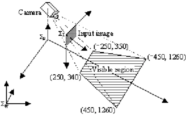
3·2 Transformation from image coordinates to environmental map coordinates
A camera captures outdoor scene with WINDOWS DIB still-images of 240x340[pixel]. Sub images of the captured DIB images are classified into an outdoor element and, furthermore, the geographical evaluation values are allocated according to the elements. Next, the captured DIB still-images are transformed from image coordinates( Σ I) to world
coordinates( ΣW), via camera coordinates( ΣC), and robot
coordinates(ΣR), and the allocated geographical evaluation
values are embedded in an environmental map.
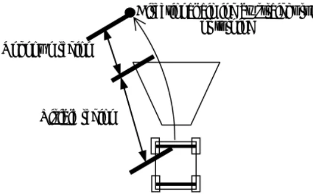
The camera is set at 210[mm] in height, and with an angle of depression of 28[degree].
Fig.4 The flow of coordinates transformation and 4 trapezoid area points onΣR [mm]
Straight or turning
Fig. 5. An example of the target path at “Approach to GOAL”
Minimum radius turning Straight
GOAL
Rmin
Fig. 6. Examples of failing in reaching GOAL GOAL
GOAL
(a) GOAL exits inner of minimum
radius turning
(b) GOAL exits at visible region
Fig. 7. Border value between “Approach to GOAL” and “Neighborhood of GOAL”
GOAL
Lbor
By performing coordinate transformation, the four-corner points on a DIB image is transformed into trapezoid area on Σ
R as shown in Fig.4. And, moreover, this trapezoid area is
transformed toΣW.
We divide the transformed picture into 16x16 pieces, and update environmental maps by embedding geographical evaluation values in environmental maps.
4. PATH PLANNING
The experimental conditions are as follows.
・The position and orientation of robot can be determined accurately enough.
・The position of GOAL is given, but the environment is unknown in advance.
・There is no obstacles that robot can't pass through such as wall and precipice.
・A robot can pass on the above-described geographical feature elements which exist in environment. But, expressing difficulty of robot’s moving, the weight coefficients for the geographical features differ.
4·1 Region definition
When using a CCD camera as a vision sensor, we find there is two kinds of areas exist. One is the area for which geographical elements can be recognized, and the other one is can not, because it is in the outside of visible area. Now, we define the former as the visible region (VR), and the latter as the unknown region (UR).
4·2 Generation of target path
As shown in Fig.5, the target path is that the robot performs turning or running straight in VR at first.
And then in UR, the robot runs the shortest length path with minimum radius turning, and running straight aiming at GOAL directly.
However, when the distance from present representation point (central point of front wheel shaft) to GOAL is not far enough, the above mentioned target path is not necessarily successfully generated. Fig.6 shows two such cases. They are the case that GOAL exists in the area of the minimum turning radius in UR, and the other case that GOAL exists in VR. Therefore, we make a little change to generation of a target path in this case.
When Lbor shown in Fig.7 satisfies
Lbor ≧ 2Rmin (3)
We define this case as "Approach to GOAL". Contrary to this, when Lbor satisfies
Lbor < 2Rmin (4)
We define this case as "Neighbor of GOAL". where
α θ k=0 k-1
k Ldev Pend XR YR
Fig. 8. Target path at visible region GOAL
Fig. 9. One of the paths at “Neighbor of GOAL” Directional aiming by straight run
or turning Unknown region
Visible region 4·3 Path planning at "Approach to GOAL"
The robot goes toward GOAL, searching the optimal path out of target pathes generated. Now, we consider a path evaluation value as a standard value for searching the optimal path. The path evaluation value expresses the grade of the difficulty of movement for a robot.
4·3·1 Calculation of path evaluation value in VR The target path is generated by changing target angle α and control angle θ, as shown in Fig.8.
α : Target angle, which is defined as an angle between the YR axis and the line segment that connects the robot
representation point and the target point being set in VR (Pend).
θ : Control angle, which is the steering angle of the robot.
The robot performs turning movement ( α ≠ θ ) or straight movement (α = θ) in VR by changing αand θ.
When the robot moves in VR, the robot searches for the optimal path based on the geographical evaluation value.
When the robot moves, the geographical features should be examined only at the places that the robot's wheel steps on.
Therefore, the robot's shape should not be represented in a generally used shapes such as a circular and a rectangle, but in the two points, that is, the left and right wheel points.
It is considered that just the geographical feature, which the two points step on, should be taken into consideration.
Once a set of α and θis given, the robot generates a target path in VR. Moving along the generated target path, the robot calculates the movement evaluation value at each of sampling step.
Movement evaluation value at a certain sampling step k,
J(k) is defined by
( )
k K J( )
k 2J( )
kJ = × L + R (5)
where
JL(k) : Geographical evaluation value, on which
robot's left wheel steps, at a sampling step k.
JR(k) : Geographical evaluation value, on which
robot's right wheel steps, at a sampling step k.
K : The weight coefficient used when right and left wheel step on different geographical feature elements.
As a result, path evaluation value in VR, Jv, by a set of α and θ is given by
(
) ( )
¦
= »¼ º «¬ ª × − + = n k dev v L J k J k J 1 2 1 (6) whereLdev : Length of the path that the robot moves along in one sampling step as shown in Fig.8.
4·3·2 Path evaluation value in UR
In UR, the robot performs the shortest distance movement, the path of which is created by concatenating the minimum rotation radius movement with the straight movement to GOAL.
When the movement evaluation value at Pend is given as Jn, the path evaluation value in UR, Ju, is given by
unk G n u J J L J = + × 2
(7)
JG : Geographical evaluation value at GOAL
(given)
Lunk : Estimated shortest length of the path, along
which robot will run in UR.
4·3·3 Total path evaluation value
Finally, the total path evaluation value Jt is given by, u
v t J J
J = + (8)
The robot repeats choosing the optimal course at every sampling time, for which a course evaluation value is the lowest, and moves toward GOAL.
4·3·4 Path planning at "Neighbor of GOAL"
At "Neighbor of GOAL", the target angle α is fixed toward GOAL direction from the robot position, and the control angle θ is changed one by one, and, thus, the target path is generated. Turning (α ≠ θ) or running straight (α = θ), the target path directly reaches at the goal as show in Fig.9.
Path evaluation value at Neighbor of GOAL is calculated by the same method that is used in Approach to GOAL.
Fig.10 Experimental result in case of far-ranging grass lies in depth direction
Fig.11 Experimental result in case of narrowly-ranging grass lies in depth direction
Fig.12 Experimental result in case of asphalt road runs up as hook form Grass Area Grass Area Grass Area Grass Area GOAL GOAL
GOAL
GOAL
GOAL
GOAL
Scale 1m Scale 1m Scale 1m 5. MOBILE ROBOT DEAD RECKONINGDead reckoning should have to minimize its unbounded growth in position and orientation errors. This can be accomplished by meticulously modeling sensor errors and by efficient filter design.
5.1 The error model for encoder
The mobile robot position and orientation are calculated from the output of incremental encoder system It is well known that system is subject to systematic errors caused by factors such as unequal wheel-diameters, imprecisely measured wheel diameters, or an imprecisely measured wheel separation distance. Subject to these errors the robot’s position and orientation angle are computed as error model.
5.2 The error model for gyro and accelerometer
Inertial navigation uses gyro sensor and acceleration sensor to measure rate of rotation and acceleration respectively. However, inertial sensor data drift with time because of the need to integrate rate data to yield position. Considering the bias drift of those sensors, the robot’s position and orientation are computed as error model.
5.3 Fusion of error model data
We use the Kalman filter tool for fusion all error measure by provided sensor. The fusion method will improve the dead-reckoning accuracy of a mobile robot based on encoder system, gyro and accelerometer. We used this mobile robot positioning method and conduct the path planning experiment using geographical information.
6. EXPERIMENT
The experimental conditions are as follows. (Refer to Path Planning in chapter 4 for more detail)
・Width of robot wheel has 282[mm] by 220[mm] length. ・Ldev is 5.0[mm] length.
・The initial stage of environment is unknown and the GOAL is given.
Experimental results are shown in Fig.10 to Fig.12. In these figures, the brighter the gray level is, the lower of the geographical evaluation value is. Contrary to this, the darker the gray level is, the higher of the geographical evaluation value is. The geographical features recognition’s also depend on the experiment time and weather condition, which the minute difference of gray level contrast will affect to geographical evaluation value. But this is not effect to the essence result. Our experiments have conducted in clear weather condition. If the geographical evaluation value is same, we set priority to robot turn right. The white area shows the regions that haven’t been capture by the camera. And all the area is unknown except the area captured by camera. The variable t represents sampling times that initiates from 0. 6·1 Far-ranging grass lies in depth direction
In Fig.10, START position is (0, 0)[mm], GOAL position is (0, 5000) [mm], rectangle Top-Left and Bottom-Right points of grassy field are (-1500, 4000) [mm] and (1500, 2000) [mm].
Under the condition, the robot detects grassy geography and detours to right. Finally, the robot turns from a left bottom corner, and successful reaches GOAL.
6·2 Narrowly-ranging grass lies in depth direction In Fig.11, START position and GOAL position are same with Fig.10, rectangle Top-Left and Bottom-Right points of grassy field are (-1500, 2230) [mm] and (1500, 2000) [mm].
Under this condition, the robot detects grassy geography and detours as it is. However, different from the case mentioned above, recognizing the grass area is narrow then the robot selects the path traversing the grass geography, and successful reaches GOAL.
6·3 Asphalt road runs up as hook form
In Fig.12, START position is (0, 0) [mm], GOAL position is (-9000, 9000) [mm], asphalt field spreads as hook form.
Under this condition, the robot detects grassy geography, and aims for GOAL along grassy field. Then, having passed the grassy geography, the robot goes straight toward GOAL. However the mobile robot again detecting another grassy geography, the robot aims for GOAL along the new grassy field. Finally, the robot successful reaches GOAL.
7. CONCLUSION
In this research, we propose the following algorithm are describe as below:
・Based on geographical information, pathes were created. The geographical information was transformed into a 1-dimensional evaluation value that expresses the difficulty of movement for the robot.
・The target path was generated by changing the target angle α and the control angle θ.
・The situations are classified into either Approach to GOAL or Neighbor of GOAL, and the path planning algorithm is switched to another one.
・The robot was assumed to be two points object. From the experimental results, we can conclude as below: ・After recognizing geographical feature, the robot performs path planning based on generated environmental map embedded geographical evaluation value, and, successfully, reaches GOAL.
・The robot passed through a grassy geography in the case that the grass area is narrowly ranging. Contrary to this, in the other case that the grassy area is far ranging, the robot escapes the grassy area.
・The robot dead reckoning by sensor fusion with error model method success to reduce the accumulated error during traveling in various geographical environments.
REFERENCES
[1] H.Noborio. "Several path Planning Algorithms of a Mobile Robot for an uncertain Workspace and Their Evaluation", Proc. of the IEEE Int. Work. Intel. Motion Control, vol.1, August 1990.
[2] V.Lumelsky, "Effect of Uncertainry on Continuous Path Planning for an Autonomous Vehicle", Proc. of the 23rd IEEE Conf. On Decision and Control, Las Vegas, Nevada, December 1984.
[3] T.Kanbara, "A Method of Planning Movement and Observation for a Mobile Robot Considering Uncertainties of Movement, Visual Sensing, and a Map", Transactions of the Japan Society of Mechanical Engineers, vol.65, no.629, 1999
[4] M.Yamada, "Autonomous Navigation of an Intelligent Vehicle Using 1-D Optical Flow", Transactions of the Japan Society of Mechanical Engineers, vol.64, no.617, 1998
[5] S.Tadokoro, "Generation of Avoidance Motion for Robots which Coexist and Cooperate with Human (2nd Report, Avoidance of Moving Obstacles for Mobile Robots)", Transactions of the Japan Society of Mechanical Engineers, vol.63, no.606, 1997
[6] S. hoichi Maeyama, Nobuyuki Ishikawa and Shin'ichi Yuta, “Rule based filtering and fusion of odometry and gyroscope for a fail safe dead reckoning system of a mobile robot’’, IEEE International Conference on Multisensor Fusion and Integration for Intelligence Systems,pp.541-548(1996.12)
[7] J. Borenstein and L. Feng, “Gyrodometry: A New Method for Combining Data from Gyros and Odometry in Mobile Robots”, Proc. Of Int. Conference on Robotics and Automation, Vol.1, pp.423-428 (2001).
[8] Shoichi Maeyama, Akihisa Ohya, and Shin’ichi Yuta, “Robust Dead Reckoning System by Fusion of Odometry and Gyro for Mobile Robot Outdoor Navigation”, Nihon Robot Journal., Vol.15, No. 8, pp.1180-1187(1997)
[9] S. .Hasegawa, "Environment Recognition by Integrated Visual Information Based on D-S theory", Proc. of IEEE International Workspace on Robot and Human Communication.
[10] Nomura, Semii, "Character Recognition for Plans Using Dempster-Shafer Theory", The Journal of The Institute of Electronics, Information and Communication Engineers, (D-Ⅱ),Vol.J79-D-Ⅱ,No.5.