ICCAS2005 June 2-5, KINTEX, Gyeonggi-Do, Korea
Unscented Filtering in a Unit Quaternion Space for Spacecraft Attitude Estimation
Yee-Jin Cheon∗∗KOMPSAT-3 System Engineering & Integration Dept., Korea Aerospace Research Institute, Daejeon 305-333, Korea
(Tel: +82-42-860-2757; Fax: +82-42-860-2007; Email:[email protected])
Abstract: A new approach to the straightforward implementation of the unscented filter in a unit quaternion space is proposed for spacecraft attitude estimation. Since the unscented filter is formulated in a vector space and the unit quaternions do not belong to a vector space but lie on a nonlinear manifold, the weighted sum of quaternion samples does not produce a unit quaternion estimate. To overcome this difficulty, a method of weighted mean computation for quaternions is derived in rotational space, leading to a quaternion with unit norm. A quaternion multiplication is used for predicted covariance computation and quaternion update, which makes a quaternion in a filter lie in the unit quaternion space. Since the quaternion process noise increases the uncertainty in attitude orientation, modeling it either as the vector part of a quaternion or as a rotation vector is considered. Simulation results illustrate that the proposed approach successfully estimates spacecraft attitude for large initial errors and high tip-off rates, and modeling the quaternion process noise as a rotation vector is more optimal than handling it as the vector part of a quaternion.
Keywords: Unscented Kalman Filter, Unit Quaternion Space, Quaternion Mean, Attitude Estimation, Rotation Vector 1. Introduction
Attitude estimation is one of the basic problems and an important issue in many spacecraft applications, and has been studied extensively in the past [5][10][14][15][16][17][18]. There are several parameterizations available for spacecraft attitude representation, such as Euler angles, quaternions, modified Rodrigues parameters, and even the rotation vec-tor. The detailed discussion on each parametrization for at-titude estimation is found in [5]. The extended Kalman fil-ter (EKF) is widely used for attitude estimation [14][15][18]. The unscented Kalman filter (UKF) is an extension of the classical Kalman filter to nonlinear process and measurement models and an alternative to the EKF for a variety of estima-tion and control problems [5][11][13][19][20]. For nonlinear systems the UKF uses a deterministically chosen minimal set of sample points to capture the probability distribution more accurately than the linearization of the EKF, result-ing in faster convergence from inaccurate initial conditions in attitude estimation problems.
In [11], the experiment which compares UKF and EKF for human head and hand orientation data represented with quaternions is presented. However, the estimated mean value is simply derived using an average sum of the quaternions by treating the quaternion as an element in vector space, which leads the quaternion estimate to depart from the unit sphere. The quaternion is normalized by brute force and the linearized model of quaternion kinematics is used, which does not take full advantage of the UKF capabilities. To di-rectly utilize UKF formulation built in vector space and to avoid a mean computation problem of quaternions, a mod-ified method employing the combination of the quaternion with the generalized Rodrigues parameters is used in [5]. This method converts a quaternion to a Rodrigues parame-ter and converted Rodrigues parameparame-ters are used to compute the predicted mean, the covariance and cross-relation matrix since Rodrigues parameters are unconstrained, i.e, lying in
vector space. Rodrigues parameters are converted back to quaternion because this method uses the inertial quaternion for state propagation. It was shown that the performance of UKF outperforms that of the standard EKF for large initial-ization errors [5].
Generally, the problem in calculating the mean of a set of ro-tations lies in the fact that roro-tations do not belong to a vector space, but lie on a nonlinear manifold. If we choose to rep-resent the rotation by a quaternion, the proper rotations are constrained to the three-dimensional unit sphere of a four-dimensional Euclidian space. In the original concept of UKF, the predicted mean is simply calculated using an averaged sum of predicted states because state vector elements lie in a vector space. However, the weighted sum of unit quaternion points, i.e, a quaternion of unit norm, does not lie on the unit sphere because unit quaternion is not mathematically closed for addition and scalar multiplication. There is no guarantee that the mean of quaternions lies on the nonlin-ear manifold with allowable rotations by directly using UKF with quaternion parameterization. Due to this fact, it seems that the direct implementation of the UKF with quaternions is undesirable. There are several research works for comput-ing means and averagcomput-ing in the group of rotations [7][8][9]. The method of averaging rotations for rotation matrices is proposed in [8]. Providing that the inner product of the quateternions is non-negative, an average of two rotations is a normalized arithmetic mean of the unit quaternions asso-ciated with the two rotations [9]. Very often the barycenter of the quaternions that represents the rotations is used as an estimate of the mean rotation. In [7], a method of averaging rotations was derived from natural approximations to the Riemannian metric to show how the barycenter mean of ro-tations approximates the mean based on Riemannian metric. By using this method, the mean rotation, i. e., the optimal quateternion, is exactly the barycenter of rotations on the curvature of the nonlinear manifold with renormalization. In this paper, a new approach to the straightforward
im-plementation of UKF with quaternion in a unit quater-nion space is proposed, where no parameter conversion is required, such as transformation between quaternions and Rodrigues parameters. To ensure that a weighted sum of quaternions lies in unit quaternion space, we derive a quaternion-based weighted mean computation method by expanding the method given in [7]. This method can be also used for the predicted observation computation when mea-surement output is given by the quaternion. To evenly dis-seminate quaternion samples on the unit sphere around the current quaternion estimate, both error quaternion and its inverse quaternion are used to generate sigma point quater-nions. A multiplicative quaternion-error is used for predicted covariance computation of the quaternion because it repre-sents the distance from the predicted mean quaternion, and the unit quaternion is not closed for subtraction, guaran-teeing that the quaternion in filter lies in unit quaternion space. To resolve the problem that a simple linear correc-tion for quaternion update makes the quaternion depart from constraint unit sphere, the quaternion is updated by multi-plication. Since quaternion process noise finally results in an increase of the uncertainty in attitude orientation, we treat the quaternion process noise as a vector part of the quater-nion or as a rotation vector.
This paper is organized as follows. A brief review of UKF is provided in Section 2.. In Section 3., a summary of attitude kinematics and the gyro model is described. The weighted mean computation method of quaternions is derived, which guarantees that the resulting quaternion has unit norm. The direct implementation of UKF with a quaternion in unit quaternion space is presented in Section 3.. In Section 4., numerical simulations for the new filter are presented using simulated three-axis magnetometer and gyro measurements. Concluding remarks follow in Section 5..
2. Unscented Kalman Filtering
The unscented Kalman filter represents a derivative-free, i.e., no need for Jacobian and Hessian calculation, alternative to the extended Kalman filter, and builds on the principle that it is easier to approximate a Gaussian distribution than it is to approximate an arbitrary nonlinear function. In the UKF, a minimal set of sample points are deterministically chosen and propagated through the original nonlinear system to capture the posterior mean and covariance of a random variable accurately to the 2nd order Taylor series expansion for any nonlinearity. More details are found in [1][2][3][4]. The general formulation of the UKF is summarized for a discrete-time nonlinear system. Let us consider the following system model of discrete-time nonlinear equations:
xk+1= f(xk, k) + wk (1a) yk= h(xk, k) + vk (1b)
where xk∈ <n×1 is the state vector, yk ∈ <m×1 is the
ob-servation vector, f and h are the nonlinear system dynamic models. It is assumed that the process noise wk and
mea-surement noise vector vk are uncorrelated white Gaussian
processes with zero means and covariances given by Qk and
Rk, respectively. Then, given an n × n covariance matrix Pk, the set of (2n + 1) sigma points Xk∈ <2n+1is computed
as follows: X0,k= ˆxk (2a) Xi,k= ˆxk+ ³ γp(Pk+ Qk) ´ i for i = 1, · · · , n (2b) Xi,k= ˆxk− ³ γp(Pk+ Qk) ´ i for i = n + 1, · · · , 2n (2c) where γ =√n + λ and λ = α2(n+κ)−n is a composite
scal-ing parameter. The constant α determines the spread of the sigma points around ˆxkand is usually set to a small positive
value (0 ≤ α ≤ 1). The constant κ is a secondary scaling parameter which is usually set to 0 or 3 − n and provides an extra degree of freedom for fine tuning of the higher order moments. The matrix square-rootp(Pk+ Qk) can be
cal-culated by a lower triangular Cholesky factorization. From Eq. (2) a matrix Xk of 2n + 1 sigma vectors Xi,k is formed
as Xk= h ˆ xk ˆxk+ γ p (Pk+ Qk) xˆk+ γ p (Pk+ Qk) i (3) The transformed sigma vectors are propagated through the following nonlinear function:
Xi,k+1= f(Xi,k, k) (4)
where Xi,k is the ith column of Xk. The predicted state
vector ˆx−k+1and its predicted covariance P −
k+1are computed
using a weighted sample mean and covariance of the posterior sigma point vectors, as follows:
ˆ x− k+1= 2n X i=0 Wi(m)Xi,k+1 (5) P−k+1= 2n X i=0 Wi(c){Xi,k+1− ˆx−k+1}{Xi,k+1− ˆx−k+1} T (6) with the following weights Wi [4]:
W0(m)= λ/(n + λ) (7a) W0(c)= λ/(n + λ) + (1 − α 2 + β) (7b) Wi(m)= W (c) i = 1/{2(n + λ)} i = 1, · · · , 2n (7c)
where β is used to make further higher order effects to be incorporated by adding the weighting of the zeroth sigma point of the calculation of the covariance (for Gaussian dis-tributions β = 2 is optimal).
Similarly, the predicted observation vector ˆy−k+1 is also
cal-culated as ˆ y− k+1= 2n X i=0 Wi(m)Yi,k+1 (8) where Yi,k+1= h(Xi,k+1, k + 1) (9)
The predicted output covariance Pyyk+1 is given by Pyy k+1= 2n X i=0
Wi(c){Yi,k+1− ˆy−k+1}{Yi,k+1− ˆy−k+1}T (10)
then the innovation covariance Pvv
k+1is calculated by Pvv
k+1= Pyyk+1+ Rk+1 (11)
The filter gain Kk+1 is computed by Kk+1= Pxyk+1(P
vv
k+1)−1 (12)
and the cross correlation matrix is obtained as
Pxyk+1=
2n
X
i=0
Wi(c){Xi,k+1− ˆx−k+1}{Yi,k+1− ˆy−k+1} T
(13) The estimated state vector ˆx+
k+1 and updated covariance P+ k+1are given by ˆ x+k+1= ˆx − k+1+ Kk+1(yk+1− ˆy − k+1) (14) P+k+1= P − k+1− Kk+1Pvvk+1Kk+1T (15)
3. Unscented Filtering in a Unit Quaternion Space The difficulty of filtering unit quaternion data stems from the nonlinear nature of unit quaternion space. In other words, the problem in calculating the mean of a set of quaternions lies in the fact that rotations represented by the quater-nion do not belong to a vector space, but lie on a nonlin-ear manifold and the quateternions are constrained to the three-dimensional unit sphere of a four-dimensional Euclid-ian space. The weighted sum of unit quaternion points is generally not a quaternion of unit norm because the unit quaternion is not mathematically closed for addition and scalar multiplication. With reference to Eq. (5), there is no guarantees that the resulting quaternion will have unit norm. Due to this fact, the straightforward implementation of the UKF with quaternions seems to be undesirable. In the original concept of UKF, the predicted mean is simply calculated using an averaged sum of predicted states, i.e., sum over all the elements of the set divided by the number of elements. This is true when the state vector elements lie in a vector space. However, if the state vector is quater-nion, the predicted quaternion mean should be calculated in the rotational space to preserve the nonlinear nature of unit quaternion. A UKF in a unit quaternion space is pos-sible when a weighted mean of quaternions produces a unit quaternion estimate, and the predicted covariance computa-tion and quaternion guarantees that quaternion in filer lies on unit sphere.
In this section, the quaternion attitude kinematics and gyro model are briefly reviewed and a UKF in unit quaternion space for attitude estimation is derived by preserving the nonlinear nature of unit quaternion space.
The attitude of spacecraft can be described by means of quaternion parameterization, defined as
q ≡ " q13 q4 # (16) with q13≡ q1 q2 q3 = ˆn sin(Φ/2) (17a) q4= cos(Φ/2) (17b)
where ˆn is a unit vector corresponding to the rotation axis
and Φ is the angle of rotation. The quaternion satisfies the following normalization constraint
qTq = qT13q13+ q42= 1 (18)
The inverse quaternion is defined as
q−1≡ h −q13 q4 iT = h −q1 −q2 −q3 q4 iT (19) The quaternion kinematic equations of motion are obtained by using angular velocity (ω) as follows
˙q =1 2Ω(ω)q (20) with Ω(ω) ≡ − [ω×] ... ω . . . ... . . . −ωT ... 0 (21)
where the matrix cross product operator [ω×] represents the skew-symmetric matrix, defined by
[ω×] = 0 −ω3 ω2 ω3 0 −ω1 −ω2 ω1 0 (22)
The measured angular rate output ˜ω is modeled as [6]
˜
ω = ω + b + η1 (23a)
˙b = η2 (23b)
where ω is the true angular rate of the spacecraft, η1 and
η2 are white Gaussian processes with zero means and b is
a gyro bias error. Given a post-update estimates ˆb+k, the
post-update of ω and b are given by ˆ ω+k = ˜ω − b + k (24a) ˆb− k+1= ˆb + k (24b)
Given post-update estimates ˆω+
k and ˆq
+
k, the quaternion can
then be propagated in the discrete-time equivalent form of Eq. (20), given by [5] ˆq−k+1= Ω( ˆω + k)ˆq + k (25) with Ω( ˆω+ k) ≡ " cos(0.5|| ˆω+ k||∆t)I3×3 ψˆk+ − ˆψ+T k cos(0.5|| ˆω+k||∆t) # (26) where ˆψ+ k = sin(0.5|| ˆω + k||∆t) ˆω + k/|| ˆω +
k|| and ∆t is the
The normalization constraint Eq. (18) deprives the quater-nion of one degree of freedom and simplifies the handling of the quaternion. However, the three degrees of freedom, i.e., vector part of the quaternion, are sufficient to represent any spatial rotation because q and −q yield identical rota-tions and the quaternion elements are no longer independent of each other. Given the vector part q13 of the quaternion,
there will be positive and negative values of q4 that satisfy
the quaternion normalization constraint. We choose the fol-lowing positive value of q4 throughout the filter formulation:
q4=
q 1 − qT
13q13 (27)
The state vector of the filter is defined as ˆ x+k ≡ " ˆ σ+ k ˆb+ k # (28) where ˆσ+
k is the vector part of the quaternion and ˆb
+
k is the
gyro bias part of the state vector.
Therefore we choose the process noise wkin Eq. (1a) with a
6-dimensional noise vector.
The set of transformed sigma points will be of the form:
Xk≡ " Xσ k Xb k # (29) where Xσ
k corresponds to the first three components of the
quaternion and Xb
k is the gyro bias part. To forwardly
propagate quaternions using Eq. (25), sigma points cor-responding to the quaternion have to be expanded to a 4 × 1 dimensional vector. The scalar part of the quater-nion is simply calculated using Eq. (27) from ˆσ+
k, i.e., ˆq+ k = h ˆ σ+ k q 1 − ˆσ+T k σˆ + k iT . Let denote γpPk+ Qk in Eq. (3) as
ζ ≡ " ζσ k ζb k # (30) where ζσ
i,k are the first 3 elements of the quaternion, and ζb
i,k are the next 3 elements corresponding to the gyro bias.
Since the role of process noise for the quaternion in Eq. (1a) increases the uncertainty in attitude orientation, the process noise for the quaternion can be modeled either as a vector part of a quaternion or as a rotation vector, both leading to orientation uncertainty in the attitude. Since the quaternion process noise is a 3-dimensional noise vector, it has to be expanded into a 4 × 1 dimensional unit quaternion to apply the multiplicative quaternion-error approach.
When the quaternion process noise is treated as a vector part of the quaternion, the noise vector is simply expanded into quaternion parametrization using Eq. (27), as follows:
δq+ i,k= h ζσ i,k q 1 − ζσT i,kζσi,k iT . (31)
To find a quaternion from a rotation vector, compute the angle from the magnitude of the rotation vector, then find the rotation axis by the dividing rotation vector by the an-gle, and then convert the angle and the rotation axis to the
quaternion. Modeling ζσ
i,k as a rotation vector leads to the
following 4 × 1 error quaternion:
δq+
i,k=
h
ζσ
i,ksin(|ζσi,k|/2)/|ζσi,k| cos(|ζσi,k|/2)
iT
(32) Since the unit quaternion is not closed for addition and sub-traction, the transformed sigma points of the quaternion are not simply constructed while the sigma points for the gyro bias are simply calculated by Eq. (3). The transformed sigma points for the quaternion are also quaternions satisfying the normalization constraints and should be scattered around the current quaternion estimate on the unit sphere. There-fore, the transformed quaternion sigma points are generated by multiplying the error quaternion by the current quater-nion estimate. To evenly disseminate quaterquater-nion samples on the unit sphere around the current quaternion estimate, both the error quaternion and the inverse of error quaternion, i.e.,
δq+i,k and (δq
+
i,k)−1, are used. The sigma point quaternions
are computed by the following equations:
X0,kq = ˆq + k (33a) Xq i,k= δq + i,k⊗ ˆq+k for i = 1, · · · , 6 (33b) Xi,kq = (δq + i,k) −1 ⊗ ˆq+k for i = 7, · · · , 12 (33c)
where ⊗ is the quaternion multiplier [21]. Then the set of 13 sigma points is constructed as
Xk0 ≡ " Xkq Xb k # = " ˆq+ k δq + k ⊗ ˆq + k (δq + k)−1⊗ ˆq + k ˆb+ k ˆb + k + ζbk ˆb + k − ζbk # (34) Now these transformed quaternions are propagated forward to k + 1 by Eq. (25) as follows:
Xq
i,k+1= Ω( ˆω
+
i,k)Xi,kq (35)
where the estimated angular rates are given by ˆ
ω+
i,k= ˜ωk− Xi,kb (36)
The weighted sum of unit quaternions is generally not a quaternion of unit norm because the unit quaternion is not mathematically closed for addition and scalar multiplication. Therefore, the predicted quaternion ˆq−
k+1is not simply
com-puted using weighted sample mean in Eq. (5). To resolve this problem, we derive a quaternion-based weighted mean com-putation method based on the formulation in [7] by consid-ering weights Wi. For two rotations represented by
quater-nions, q and q0, we define a distance metric d(q, q0) that
rep-resents the distance along a curve on the manifold because the vectorial distance ||q−q0|| takes no account of the
curva-ture of manifold. The distance metric between two rotations represented by quaternions is defined using the quaternion multiplication as follows: d(q, q0) = θ(q−1⊗ q0) (37a) = θ((q4q130 − q 0 4q13− q13× q 0 13, q · q 0 )) (37b) = 2 arccos(q · q0) (37c)
where θ(·) is the angle of rotation produced by the quater-nions. From classical geometry, the geodesics on a sphere
are formed by the great circles and the distance between two points on the unit sphere is therefore the angle between the corresponding vectors [7]. Ignoring the difference in scale, the distance between quaterions is exactly given by Eq. (37). As shown in Eq. (37), the distance between two rotations represented by quaternions is nonlinear function of vectorial representation. We linearize Eq. (37) to compute a closed form approximation of the mean. The following Taylor ex-pansion of cosine is used:
cos(θ 2) = 1 −
1 8θ
2+ o(θ4) (38)
Rearranging this expression yields
θ2(q−1⊗ q0) = 8 µ 1 − cos µ θ(q−1⊗ q0) 2 ¶¶ + o(θ4) (39a) ≈ 8(1 − q · q0) (39b)
The mean rotation is now the following quaternion q that minimizes the quadratic cost function [7]:
E2=
Ne
X
i=1
θ2(q−1⊗ qi) (40)
where Ne is the number of quaternion samples. Using the
approximation in Eq. (39b), the quaternion mean ¯q with weights Wiis determined as ¯q = arg min |q|=1 Ne X i=1 Wiθ2(q−1⊗ qi) (41a) ≈ arg min |q|=1 Ne X i=1 8Wi(1 − q · qi) (41b) = arg max |q|=1 Ne X i=1 Wiq · qi= arg max|q|=1q · Ne X i=1 Wiqi (41c) = PNe i=1Wiqi ¯ ¯ ¯PNe i=1Wiqi ¯ ¯ ¯ (41d) The quaternion mean computed by Eq. (41d) is the barycen-tric mean with renormalization. It should be noted that renormalization is obtained by the true optimization of an approximated cost function and not an ad hoc repair of an approximated optimization.
Now the predicted quaternion ˆq−
k+1 is computed using
Eqs. (7a), (7c), (35) and (41d) as follows: ˆq−k+1= P12 i=0WiX q i,k+1 ¯ ¯ ¯P12i=0WiX q i,k+1 ¯ ¯ ¯ (42) Since the quaternion samples are not distributed over all the unit sphere but scattered around the mean quaternion, the predicted quaternion produces a good approximation com-pared to the mean based on the Riemannian metric. For ζσ
i,k with small values the quaternion process noise, i.e.,
error quaternion given by Eq. (32), is approximated by
δq+i,k = h ζσ i,k/2 q 1 − ζσT i,kζσi,k/4 iT (43) Comparing this result with Eq. (31), the orientation uncer-tainty induced by the process noise modeled as the rotation
vector is less than that produced by modeling the process noise as the vector part of a quaternion. In other words, the transformed sigma points for the process noise modeled as the vector part of a quaternion are more widely scat-tered around the current estimate than that for the process noise treated as a rotation vector. The propagated quater-nion samples using Eq. (25) produce the same situation, i.e., the process noise of the rotation vector yields samples with smaller distances from the mean compared to the case where the process noise is modeled as the vector part of a nion. Since the approximation is used to derive the quater-nion mean given by (41d), samples with smaller distances from the mean yield better approximation of the true mean. Therefore the process noise modeled as the rotation vector will produce better results over the case where it is modeled as the vector part of a quaternion. The performance com-parison between both process models is made in Section 4.. The predicted covariance of posterior quaternions can not be directly computed using Eq. (6) because the unit quaternion is not closed for subtraction. We can use the error quater-nion for predicted covariance computation because it repre-sents the distance from the predicted mean quaternion ˆq−
k+1.
The error quaternion for predicted covariance computation is given by Λi= Xi,k+1q ⊗ [ˆq − k+1] −1 i = 0, 1, · · · , 12 (44) Since state vector of the filter includes the vector part of the quaternion, the predicted covariance for the quaternion is then computed as Pq−k+1= 12 X i=0 Wi(c)Λ 0 iΛ 0T i (45)
where Λ0iare the first three components of Λi.
The weighted quaternion averaging method can be used again for the predicted observation computation when the measurement model is given by the quaternion, such as a star tracker quaternion output. The predicted measurement co-variance is computed for such an output measurement model using Eq. (45) with Λi. The cross correlation matrix for the
quaternion is given by Pqyk+1= 12 X i=0 Wi(c)Λ 0 i{Yi,k+1− ˆy−k+1} T (46) Simple linear correction applied to quaternion update as in Eq. (14) makes the quaternion depart from the constraint unit sphere. To solve this problem, the quaternion is updated by multiplication. The estimated quaternion ˆq+
k+1 is given by ˆq+ k+1= δq+k+1⊗ ˆq−k+1 (47) where δq+ k+1≡ h δq+ 13 δq + 4 iT is represented by δq+13= Kk+1(yk+1− ˆy − k+1) (48a) δq4+= q 1 − δq+T 13 δq+13 (48b)
4. Numerical Simulations
In this section, numerical simulations for the new filter are presented using simulated three-axis magnetometer (TAM) and gyro measurements of KOMPSAT-1 (Korea Multi-Purpose Satellite-1) which was launched in 1999 and is still flying in space. The mission orbit of KOMPSAT-1 is a sun-synchronous circular obit with altitude 685.13km. Or-bit inclination is 98.13 deg and eccentricity is 0 to 0.001. The satellite operates in a nominal 10:50 AM +10/-15 min-utes local time of ascending node. Since the main mission of KOMPSAT-1 is earth observation, the nominal mission mode is earth-pointing requiring a rotation once per orbit about the spacecraft’s pitch axis, i.e., y axis. Here we only considered TAM and gyro measurements for attitude estima-tion. Inertial magnetic filed vectors were modeled using the 10th-order International Geomagnetic Reference Field model [22]. Measurement noise of the TAM was modeled by a zero mean white Gaussian process with a standard deviation of 100 nT. The gyroscopic measurements were simulated with an initial bias of 0.1 deg/h for each axis. The gyro and TAM measurements were both sampled at a 1 second interval. The simulations were performed for both process noise cases, i.e., vector part of a quaternion and rotation vector, under the same situations.
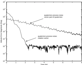
In the first simulation, we considered the nominal earth pointing mode. Errors of -180, -60, and 180 deg for roll, pitch, and yaw axis, respectively, were added into the ini-tial condition of the attitude estimate, with an iniini-tial bias estimate of 0 deg/h for each axis. Figure 1 depicts the norm of attitude errors for this simulation case. The process noise modeled as a vector part of a quaternion took almost 8 hours to reach 0.1 deg, whereas a rotation vector treated as the process noise reached this value in 1.5 hours. Finally it converged to a value of 0.001 deg within 2.5 hours. When there is large uncertainty in the initial estimates, the results indicate that the process noise as a rotation vector yields much better performance over the case where it is handled as a vector part of quaternion.
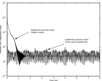
In the second simulation, a tumbling situation after separa-tion from launch vehicle was considered. Attitude estimasepara-tion is not so easy in tumbling situation because initial attitude errors are generally large and angular velocity of each axis is much higher than that of the earth pointing mode. The max-imum allowable tip-off rate for KOMPSAT-1 was 2 deg/sec about an arbitrary axis. Tip-off rates of 2, -2, and 2 deg/sec, respectively, were set with initial bias of 0.1 deg/h for each axis. A plot of the norm of attitude errors of spacecraft’s tumbling case is shown in Figure 2. The attitude errors did not reach the value obtained in the nominal earth pointing mode because angular velocity of each axis is much larger than that of the earth pointing mode, leading to rapid at-titude changes. However, we can see that the process noise modeled as a rotation vector produces better performance over the case for which it is formulated as a vector part of quaternion. The filter treating rotation vector as the pro-cess noise reduces the attitude error of 0.2 deg, whereas the attitude error for the process noise handled as a vector part
of quaternion remains within error bounds of 1 deg. Com-paring to the result of the first simulation for the process noise as vector part quaternion, the attitude error of 0.2 deg is acceptable in the tumbling mode. This simulation re-sult illustrates that attitude estimation in tumbling mode is achieved with some degree of error bounds, and the process noise in the form of rotation vector produces better result compared to the case where it is modeled as vector part of quaternion.
From simulations, it can be said that in the presence of large uncertainties in the initial conditions and in the situation of high tip-off rates, the process noise as a rotation vector is more optimal than modeling it as a vector part of quater-nion.
5. Conclusions
In this paper a new approach to the straightforward imple-mentation of UKF for spacecraft attitude estimation in unit quaternion space was presented. Since the UKF formula-tion is built in vector space, weighted mean computaformula-tion for quaternions did not produce an estimate in unit quaternion space. To solve this problem, weighted mean computation method for quaternions in rotational space was derived. The quaternion multiplication was used for predicted covariance computation and quaternion update, which makes quater-nion in the filter lie in unit quaterquater-nion space. To evenly scatter the quaternion samples on the unit sphere around the current quaternion estimate, both error quaternion and its inverse quaternion were used to construct sigma point quaternions. Numerical simulation results showed that the proposed approach successfully estimates attitude of space-craft for large initial errors and high tip-off rates. Since the process noise for quaternion resulted in increase of the uncer-tainty in attitude orientation, either modeling it as a vector part of quaternion or as a rotation vector was considered. From simulation results, modeling the quaternion process noise as a rotation vector is more optimal than treating it as a vector part of quaternion.
0 1 2 3 4 5 6 7 8 10−5 10−4 10−3 10−2 10−1 100 101 102 103 Time (Hr)
Attitude Error Magnitude (Deg)
quaternion process noise: vector part of quaternion
quaternion process noise: rotation vector
0 1 2 3 4 5 6 7 8 10−2 10−1 100 101 102 103 Time (Hr)
Attitude Error Magnitude (Deg)
quaternion process noise: vector part of quaternion quaternion process noise:
rotation vector
Fig. 2. Attitude Estimation Errors: Tumbling Mode.
References
[1] S. J. Julier, “The Scaled Unscented Transformation,”
Proceedings of the American Control Conference,
Amer-ican Automatic Control Council, Evanston, IL, 2002, pp. 1108–1114.
[2] S. J. Julier, J. K. Uhlmann, and H. F. Durrant-Whyte, “A New Method for the Nonlinear Trasnformation of Means and Covariances in Filters and Estimators,”
IEEE Transaction on Automatic Control, Vol. AC-45,
No. 3, 2000, pp. 477–482.
[3] S. J. Julier, and J. K. Uhlmann, “A New Extension of the Kalman Filter to Nonlinear Systems,” Signal
Processing, Sensor Fusion, and Target Recognition VI,
edited by I. Kadar, Proceedings of the SPIE, Vol. 3068, Society of Photo-Optical Instrumentation Engineers, Bellingham, WA, 1997, pp. 182–193.
[4] E.A. Wan, and R. van der Merwe, “The Unscented Kalman Filter,” Kalman Filtering in Neural Networks, edited by S. Haykin, Wiley, New York, 2001, Chap. 7. [5] J. L. Crassidis, and F. L. Markley, “Unscented Filtering
for Spacecraft Attitude Estimation,” Journal of
Guid-ance, Control and Dynamics, Vol. 26, No. 4, 2003, pp.
536–542.
[6] R. L. Farrenkopf, “Analytic Steady-State Accuracy So-lutions for Two Common Spacecraft Attitude Estima-tors,” Journal of Guidance, Control and Dynamics, Vol. 37, No. 1, 1978, pp. 282–284.
[7] C. Gramkow, “On Averaging Rotations,” International
Journal of Computer Vision, Vol. 42(1/2), 2001, pp.
7–16.
[8] M. Moakher, “Means and Averaging in the Group of Rotations,” SIAM Journal on Matrix Analysis and
Ap-plications, Vol. 24, No. 1, 2002, pp. 1–16.
[9] W. D. Curtis, A. L. Janin, and K. Zikan, “A Note on Averaging Rotations,” Virtual Reality Annual
Interna-tional Symposium, IEEE, Sept. 1993, pp. 377–385.
[10] J.-W. Kim, J. L. Crassidis, S.R. Vadali, and A.L. Der-showitz, ”International Space Station Leak Localiza-tion Using Attitude Disturbance EstimaLocaliza-tion,” IEEE
Aerospace Conferences, Big Sky, Montana, 2003,
#01-3475.
[11] J. J. LaViola, ”A Comparison of Unscented and Ex-tended Kalman Filtering for Estimating Quaternion Motion”, In the Proceedings of the 2003 American
Con-trol Conference, IEEE Press, June 2003, pp. 2435–2440.
[12] F. D. Busse, ”Demonstration of Adaptive Extended Kalman Filter for Low Earth Orbit Estimation Using DGPS”, Institute of Navigation GPS Meeting, Sept. 2002.
[13] D.-J. Lee, and K. T. Alfriend, ”Adaptive Sigma Point Filtering for State and Parameter Estimation”,
AIAA/AAS Astrodynamics Specialist Conference and Exhibit, Providence, Rhode Island, August 16–19, 2004.
[14] F. L. Markley, “Attitude Error Representation for Kalman Filtering,” Journal of Guidance, Control and
Dynamics, Vol. 26, No. 2, 2003, pp. 311–317.
[15] E. J. Lefferts, F. L. Markley, and M. D. Shuster, “Kalman Filtering for Spacecraft Attitude Estimation,”
Journal of Guidance, Control and Dynamics, Vol. 5, No.
5, 1982, pp. 417–429.
[16] J. L. Crassidis, and F. L. Markley, “Attitude Estima-tion Using Modified Rodrigues Parameters,”
Proceed-ings of the Flight Mechanics/Estimation Theory Sympo-sium, NASA Goddard Space Flight Center, Greenbelt,
MD, May 1996, pp. 71–83.
[17] N. J. Kasdin, “Satellite Quaternion Estimation from Vector Measurement with the Two-Step Optimal Es-timator,” American Astronautical Society, AAS Paper 02-002, Feb. 2002.
[18] M. L. Psiaki, “Attitude-Determination Filtering via Ex-tended Quaternion Estimation,” Journal of Guidance,
Control and Dynamics, Vol. 23, No. 2, 2000, pp. 206–
214.
[19] S. J. Julier, and H. F. Durrant-Whyte, “Navigation and Parameter Estimation of High Speed Road Vehicles,”
Robotics and Automation Conference, 1995, pp. 101–
105.
[20] B. Stenger, P. R. S. Mendonca, and R. Cipolla, “Model-Based Hand Tracking Using an Unscented Kalman Fil-ter,” Proceedings of the British Machine Vision
Confer-ence, Sept. 2001, pp. 63–72.
[21] M. D. Shuster, “A Survery of Attitude Representa-tions,” Journal of the Astronautical Sciences, Vol. 41, No. 4, 1993, pp. 439–517.
[22] C. E. Barton, “ International Geomagnetic Reference Field: The Seventh Generation,” Journal of